Intro to 1-way ANOVA: impacts of diet on deer antlers
Nathan Brouwer brouwern@gmail.com @lobrowR
2018-06-20
Source:vignettes/ANOVA_deer_antlers.Rmd
ANOVA_deer_antlers.RmdIntroduction
The purpose of this lab is to learn the basics of 1-way ANOVA in R. We will explore data where white-tailed deer where fed different diets over the course of the spring and summer of one year.
- Diet 1: “Hi.Hi” = deer fed high protein diets during spring and summer
- Diet 2: “Hi.Lo” = deer fed high quality diets during spring, but low quality diet during summer
- Diet 3: “Lo.Hi” = deer fed low-protein diet during spring but high quality diet during summer.
Note: there is no “Lo.Lo” treatment
Analyis with 1-way ANOVA will allow us to determine whether
- All of the means are similar or if at least one differs
- Which treatment, if any, is most likely impacting antler growth.
Part 1: Summary stats & plotting means
1) Summary stats on all data
In this section the grand mean on ALL the data is calculated; data is NOT broken up by treatment! Data is considered by subgroup below
Load data
library(wildlifeR)
data(antlers)
# total sample size (all observations)
dim(antlers)## [1] 30 5n.total <- length(antlers$mass)
#mean of ALL samples
summary(antlers)## diet mass circum beam
## Hi.Hi:10 Min. :346.0 Min. : 57.95 Min. :247.3
## Hi.Lo:10 1st Qu.:526.9 1st Qu.: 87.85 1st Qu.:392.9
## Lo.Hi:10 Median :648.4 Median : 96.67 Median :424.5
## Mean :635.9 Mean : 99.43 Mean :412.0
## 3rd Qu.:762.4 3rd Qu.:112.17 3rd Qu.:440.2
## Max. :919.3 Max. :136.06 Max. :568.2
## spread
## Min. :223.8
## 1st Qu.:295.1
## Median :346.0
## Mean :341.4
## 3rd Qu.:383.5
## Max. :459.7mean(antlers$mass)## [1] 635.9164#variance of ALL samples
var(antlers$mass)## [1] 25767.67#stdev of ALL samples
mass.sd <- sd(antlers$mass)2) Standard error for all data
This ignores treatments. All data are combined / pooled.
We’ll do this a couple different ways to show how R code can vary.
Broken up into steps, saving an object at each stuep
#square root of N
sqrt.n <- sqrt(n.total)

#the see
mass.se <- mass.sd/sqrt.n

mass.se
## [1] 29.30738Doing it a little “on fly”
mass.se <- mass.sd/sqrt(n.total)Totally on the fly - nothing pre-saved as an object
#Using raw data
mass.se <- sd(antlers$mass)/
             sqrt(length(antlers$mass))
3) 95% CI for all data
This is the 95% confidence interval around the overall/grand mean. W approximate the CI as 1.96*SE
1.96*mass.se## [1] 57.442464) Calcualte summary stats for each group
- Calculae the mean for each diet treatment using dplyr.
- THe group_by() function split it up by treatment
- summarize() calcualtes the mean
- Recall the “%>%” is called a “pipe”
See pages 70-73 in “Getting started with R: An INtroduction for Biologists” for information on summarize() and group_by(). In particular see section 3.7.3 on page 72: “Method 2: Pipe, no nesting”
library(dplyr)

antlers %>% group_by(diet) %>%
   summarize(mass.mean = mean(mass))
## # A tibble: 3 x 2
## diet mass.mean
## <fct> <dbl>
## 1 Hi.Hi 606.
## 2 Hi.Lo 562.
## 3 Lo.Hi 740.We can get the SD like this
antlers %>% group_by(diet) %>%
   summarize(mass.sd = sd(mass))
## # A tibble: 3 x 2
## diet mass.sd
## <fct> <dbl>
## 1 Hi.Hi 155.
## 2 Hi.Lo 135.
## 3 Lo.Hi 148.And the sample size like this
antlers %>% group_by(diet) %>%
   summarize(mass.N = length(mass))
## # A tibble: 3 x 2
## diet mass.N
## <fct> <int>
## 1 Hi.Hi 10
## 2 Hi.Lo 10
## 3 Lo.Hi 10We can calcualte all of them like below. this time we’ll store the ouptut in an object “mass.means”
mass.means <- antlers %>% group_by(diet) %>%
   summarize(mass.mean = mean(mass),
             mass.sd = sd(mass),
             mass.N = length(mass))
5) Calcualte the 3 SE values
mass.SEs <- mass.means$mass.sd/sqrt(mass.means$mass.N)Add them to the dataframme
mass.means$mass.SEs <- mass.SEsWe can conver these to approximately 95% confidence intervals like this
mass.means$mass.CI95 <- mass.means$mass.SEs*1.96What do you notice about the relationship between the SD, SE, and 95% CI?
6) Plot the 3 mean values
We’ll plot means using ggpubr. We’ll give the function ggerrorplot() the raw data and it will calculate the means etc to make the plot.
See the link below for more information http://www.sthda.com/english/articles/24-ggpubr-publication-ready-plots/79-plot-meansmedians-and-error-bars/
mean_se mean_sd mean_range
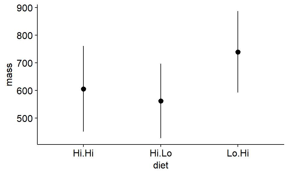
First, we’ll plot the means and their standard deviations SD
library(ggpubr)

ggerrorplot(antlers,
            x = "diet",
            y = "mass",
            desc_stat = "mean_sd",
            add = "mean"
            )
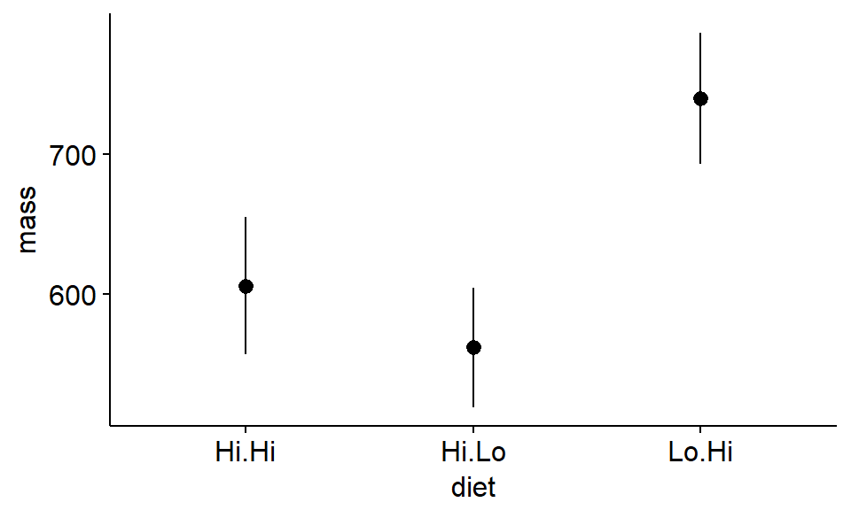
Next we’ll plot the standard errors. What happens to the x-axis?
ggerrorplot(antlers,
            x = "diet",
            y = "mass",
            desc_stat = "mean_se",
            add = "mean"
            )
We can make a plot with both if we save the plots to R objects. We’ll use the argument ylim = c(400,1000) to make it so they both have the same y axes
Note: We’ll need to load the gridExtra package
library("gridExtra")
plot1 <- ggerrorplot(antlers,
            x = "diet",
            y = "mass",
            desc_stat = "mean_sd",
            add = "mean",
            ylim = c(400,900) #set axes
            )

plot2 <- ggerrorplot(antlers,
            x = "diet",
            y = "mass",
            desc_stat = "mean_se",
            add = "mean",
            ylim = c(400,900) #set axes
            )
Plot both plots. What do you notice about the standard errors?
grid.arrange(plot1,plot2)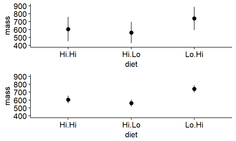
We can also easily make a plot using confience intervals.
ggerrorplot(antlers,
            x = "diet",
            y = "mass",
            desc_stat = "mean_ci",
            add = "mean",
            ylim = c(400,900) #set axes
            )
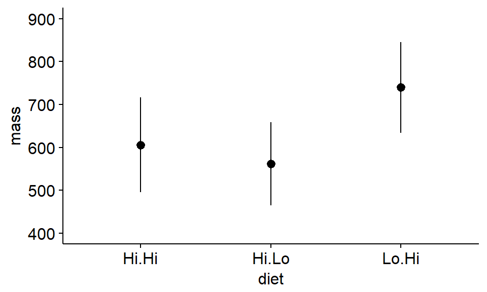
We have not calculated any p-values yet, but can you use the “inference by eye” approach to judge whether any of the means are likely to be “significantly” different based on the 95% confidence intervals?
Part 2: Omnibus ANOVA test
An “omnibus ANOVA test” (or “omnibus F test”) is used to gauge whether all the means are approximatley equal or whether at least one is likely to be different than the others. “Omnibus” means “overall”.
7 & 8) Build the null (Ho) and alternative (Ha) models
We build a null modle represent the null hypothesis that there is no difference between the any of the groups. Not that we code “mass ~ 1” to represent this null model, which has just a single mean value for all of the data.
model.null <- lm(mass ~ 1,
                 data = antlers)
We build an alternative model or “model of interest” to test the hypothesis we are interested in: that diet impacts antler growth in some way. This model will have 3 means: one for each treatment.
model.alt <- lm(mass ~ diet,
                 data = antlers)
9-12) Conduct the Omnibus test and get the ANOVA output
Produce the ANOVA table using the anova() command. This will give us the F statistics (the test statistics for ANOVA), degrees of freedom, and our p-values. (It will also give us some other info that we’ll ignore for now but that is typically reported when you do an ANOAV)
anova(model.null,
      model.alt)
## Analysis of Variance Table
##
## Model 1: mass ~ 1
## Model 2: mass ~ diet
## Res.Df RSS Df Sum of Sq F Pr(>F)
## 1 29 747262
## 2 27 575719 2 171543 4.0225 0.02958 *
## ---
## Signif. codes: 0 '***' 0.001 '**' 0.01 '*' 0.05 '.' 0.1 ' ' 1OPTIONAL:
If you are curious and things are going well, do the optional activities. These are completely optional
Optional: The summary command on an lm() object
Look at the output and how it compares to what we did with anova() on the two models.
summary(model.null)##
## Call:
## lm(formula = mass ~ 1, data = antlers)
##
## Residuals:
## Min 1Q Median 3Q Max
## -289.9 -109.0 12.5 126.5 283.4
##
## Coefficients:
## Estimate Std. Error t value Pr(>|t|)
## (Intercept) 635.92 29.31 21.7 <2e-16 ***
## ---
## Signif. codes: 0 '***' 0.001 '**' 0.01 '*' 0.05 '.' 0.1 ' ' 1
##
## Residual standard error: 160.5 on 29 degrees of freedomsummary(model.alt)##
## Call:
## lm(formula = mass ~ diet, data = antlers)
##
## Residuals:
## Min 1Q Median 3Q Max
## -322.09 -103.31 14.16 99.22 313.33
##
## Coefficients:
## Estimate Std. Error t value Pr(>|t|)
## (Intercept) 605.97 46.18 13.123 3.12e-13 ***
## dietHi.Lo -43.98 65.30 -0.673 0.5064
## dietLo.Hi 133.83 65.30 2.049 0.0503 .
## ---
## Signif. codes: 0 '***' 0.001 '**' 0.01 '*' 0.05 '.' 0.1 ' ' 1
##
## Residual standard error: 146 on 27 degrees of freedom
## Multiple R-squared: 0.2296, Adjusted R-squared: 0.1725
## F-statistic: 4.022 on 2 and 27 DF, p-value: 0.02958Optional: The anova command on a single lm() object
Look at the output and how it compares to what we did with anova() on the two models.
anova(model.alt)## Analysis of Variance Table
##
## Response: mass
## Df Sum Sq Mean Sq F value Pr(>F)
## diet 2 171543 85772 4.0225 0.02958 *
## Residuals 27 575719 21323
## ---
## Signif. codes: 0 '***' 0.001 '**' 0.01 '*' 0.05 '.' 0.1 ' ' 1Optional: Change how model is defined
We’ll add a “-1” to the model statemnt and call summary(). How does this differe from summary(model.alt)? (The difference is subtle…)
model.alt.2  <- lm(mass ~-1 + diet, data = antlers)

summary(model.alt.2)
##
## Call:
## lm(formula = mass ~ -1 + diet, data = antlers)
##
## Residuals:
## Min 1Q Median 3Q Max
## -322.09 -103.31 14.16 99.22 313.33
##
## Coefficients:
## Estimate Std. Error t value Pr(>|t|)
## dietHi.Hi 605.97 46.18 13.12 3.12e-13 ***
## dietHi.Lo 561.99 46.18 12.17 1.80e-12 ***
## dietLo.Hi 739.80 46.18 16.02 2.59e-15 ***
## ---
## Signif. codes: 0 '***' 0.001 '**' 0.01 '*' 0.05 '.' 0.1 ' ' 1
##
## Residual standard error: 146 on 27 degrees of freedom
## Multiple R-squared: 0.9553, Adjusted R-squared: 0.9503
## F-statistic: 192.3 on 3 and 27 DF, p-value: < 2.2e-16Optional: Plotting model diagnostics
We can plot the “model diagnostics” using plot(). We will go into further details on this topic in the future.
Note: the par(mfrow = c(2,2)) is a bit of cryptic R code that sets up the plotting window to have 4 panels
Also note: we’ll use the ggplot2 addon library ggfortify for this, which has a fabulous function autoplot()
#load the library
library(ggfortify)

#plot the residuals
autoplot(model.alt)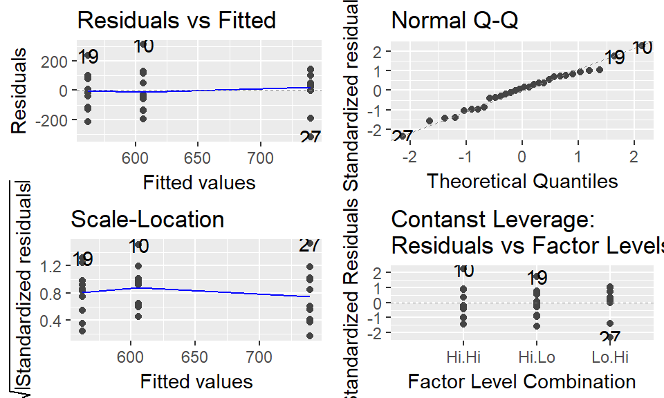
Part 3: Pairwise comparisons
The traditional way of doing a 1-way ANOVA is to follow up a “significant” Omnibus test with seperate t-tests that compare pair of means. This is called doing “pairwise” comparison - you go pair by pair doing t-tests.
The function pairwise.t.test() is used. Note that p.adjust.method = “none” line, which means we are given raw p-values that have not been corrected fro muotipel comparisons (see below)
Part 4: Pairwise comparisons, correcting for multiple comparisons, & effect sizes
The more t-tests you do, the more likely you are to get a “Significant” (low) p-value just due to chance. Rememeber - the definition of a p-value is such that it always leaves open the possiblity that the patterns you see are just due to random noise. This is called the “problem of multiple comparisons.”
One way that is advocated to to deal with this issue of multiple comparisons is to increase p-values. One way of doing this this is to use a “Bonferroni” correction. This can be done using pairwise.t.test() and setting p.adjust.method = “bonferroni”
pairwise.t.test(x = antlers$mass,
                g = antlers$diet,
                p.adjust.method = "bonferroni")
##
## Pairwise comparisons using t tests with pooled SD
##
## data: antlers$mass and antlers$diet
##
## Hi.Hi Hi.Lo
## Hi.Lo 1.000 -
## Lo.Hi 0.151 0.034
##
## P value adjustment method: bonferroni17) Build model with aov() function
When doing a 1-way ANOVA with three groups, a good option is to do a Tukey Test using the TukeyHSD() function. However, to do this you need first need to jump through a hoop: you need to redo the model model using the aov() function. (aov stands for “analysis of variance”)
model.alt.aov <- aov(mass ~ diet,
                     data = antlers)
18) Get p-values with Tukey’s HSD
When the model is fit using aov() you can then use TukeyHSD(). This gives you p-values for each set of pairwise comparisons and, more importantly effect sizes and their confidence intervals for each comparison. Importantly, the p-values and CIs have been increased to deal with the fact that you are making multiple comparisons.
TukeyHSD(model.alt.aov)## Tukey multiple comparisons of means
## 95% family-wise confidence level
##
## Fit: aov(formula = mass ~ diet, data = antlers)
##
## $diet
## diff lwr upr p adj
## Hi.Lo-Hi.Hi -43.97973 -205.89517 117.9357 0.7807326
## Lo.Hi-Hi.Hi 133.83308 -28.08236 295.7485 0.1198088
## Lo.Hi-Hi.Lo 177.81281 15.89737 339.7282 0.029204619) Plot effect sizes
The wildlifeR package contains a function that makes nice plots (IMHO) of the output of the TukeyHSD function.
par(mfrow = c(1,1))

tukey.out <- TukeyHSD(model.alt.aov)

plotTukeysHSD(tukey.out)
abline(h = 0, col = 2, lty = 2)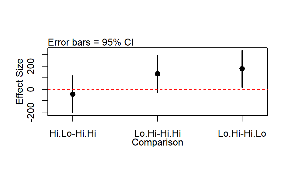
Summary of modeling workflow
First, we plot the means of the data with error bars
ggerrorplot(antlers,
            x = "diet",
            y = "mass",
            desc_stat = "mean_ci",
            add = "mean",
            ylim = c(400,900) #set axes
            )
Next, we fit a null and alternative model with the lm()
model.null <- lm(mass ~ 1, data = antlers)

model.alt <- lm(mass ~ diet, data = antlers)
THen, we compare these two models with the anova() command
anova(model.null,
      model.alt)
## Analysis of Variance Table
##
## Model 1: mass ~ 1
## Model 2: mass ~ diet
## Res.Df RSS Df Sum of Sq F Pr(>F)
## 1 29 747262
## 2 27 575719 2 171543 4.0225 0.02958 *
## ---
## Signif. codes: 0 '***' 0.001 '**' 0.01 '*' 0.05 '.' 0.1 ' ' 1We can interpret the P-value for this. We can also carry out a Tukey’s HSD test to calcualte effect sizes with confidence intervals corrected for multiple comparisons
First we have to re-fit the model with the aov() command
model.alt.aov <- aov(mass ~ diet,
                     data = antlers)
Then we use TukeyHSD() on it (note it is Tukey, NOT Tukeys w/ an “s”)
TukeyHSD(model.alt.aov)## Tukey multiple comparisons of means
## 95% family-wise confidence level
##
## Fit: aov(formula = mass ~ diet, data = antlers)
##
## $diet
## diff lwr upr p adj
## Hi.Lo-Hi.Hi -43.97973 -205.89517 117.9357 0.7807326
## Lo.Hi-Hi.Hi 133.83308 -28.08236 295.7485 0.1198088
## Lo.Hi-Hi.Lo 177.81281 15.89737 339.7282 0.0292046If I were to write this up in a paper I would say something like this:
There was a significant impact of the diet treatment on the mass of deer antlers in the experiment (F = 4.02, P = 0.03). There was no significant difference between the “Hi-lo” and “Hi-Hi” diets (Effect Size = -44, Tukey’s HSD 95% CI for effect size = -206 to 118; p = 0.8) nor was there a difference between the Lo.Hi and the Hi.Hi. treatment (Effect size = 133, 95% CI = -28 to 296, p = 0.13). The only significant difference was between the Hi.Lo and the Lo.Hi diet (Effect Size = 178, 95% CI = 16 to 340, p = 0.029).
Exploring regression with the antler data
The antler data has several response (y) variables: mass, circumference, beam length and spread. We can use regression to use one variable to predict the others.
Let’s say we want to use the beam length (the straight part of the antler from the base of the skull to where the points branch) to predict the mass.
The word equation would be mass ~ circum
We could make the scatterplot with a regression line like this
ggscatter(data = antlers,
          y = "mass",
          x = "beam",
          add = "reg.line")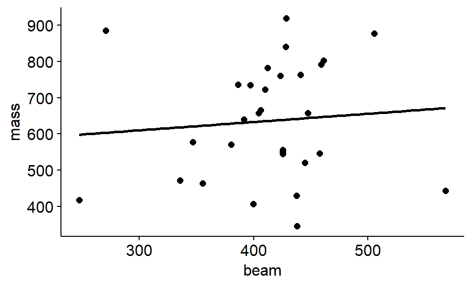
HOw do we interpret the confidence interval aroudn this plot? What do we predict the p value to be approxmatley for this regression line?
ggscatter(data = antlers,
          y = "mass",
          x = "beam",
          add = "reg.line",
          conf.int = TRUE)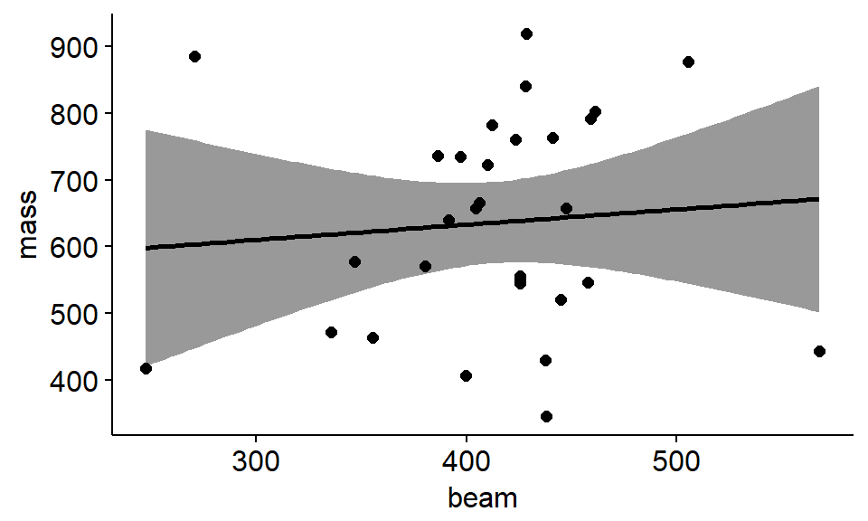
The regression code for a null model would be
mass.vs.beam.null <- lm(mass ~ 1, data = antlers)The alternative hypothesis would be represented by the model:
mass.vs.beam.alt <- lm(mass ~ beam, data = antlers)We can compare these models with the anova() command
anova(mass.vs.beam.null,
      mass.vs.beam.alt)
## Analysis of Variance Table
##
## Model 1: mass ~ 1
## Model 2: mass ~ beam
## Res.Df RSS Df Sum of Sq F Pr(>F)
## 1 29 747262
## 2 28 741623 1 5639.1 0.2129 0.6481We can get the details of the regression line using the summary() command on the alternative model
summary(mass.vs.beam.alt)##
## Call:
## lm(formula = mass ~ beam, data = antlers)
##
## Residuals:
## Min 1Q Median 3Q Max
## -295.82 -116.91 10.78 121.10 280.90
##
## Coefficients:
## Estimate Std. Error t value Pr(>|t|)
## (Intercept) 542.0213 205.6510 2.636 0.0135 *
## beam 0.2279 0.4939 0.461 0.6481
## ---
## Signif. codes: 0 '***' 0.001 '**' 0.01 '*' 0.05 '.' 0.1 ' ' 1
##
## Residual standard error: 162.7 on 28 degrees of freedom
## Multiple R-squared: 0.007546, Adjusted R-squared: -0.0279
## F-statistic: 0.2129 on 1 and 28 DF, p-value: 0.6481If I were writing up these results I would say something like this:
“THere was a positive relationship between beam length and antler mass (slope = 0.22, SE = 0.49) but the relationship was not significant (F = 0.2, p = 0.6). The model was a very poor fit to the data and explained almost no variation in the data (R^2 = 0.008)”