Original data had lat and long for most sites. Elevations estimate using the elevatr package (https://cran.r-project.org/web/packages/elevatr/vignettes/introduction_to_elevatr.html)
pikas
Format
A data frame
- lat
latitude of survey site
- long
longitude of survey site
- pika.pres
Are pikas present or absent from the site
- marmot.pres
Are marmots present or absent
- talus.area
Description of area of talus at site
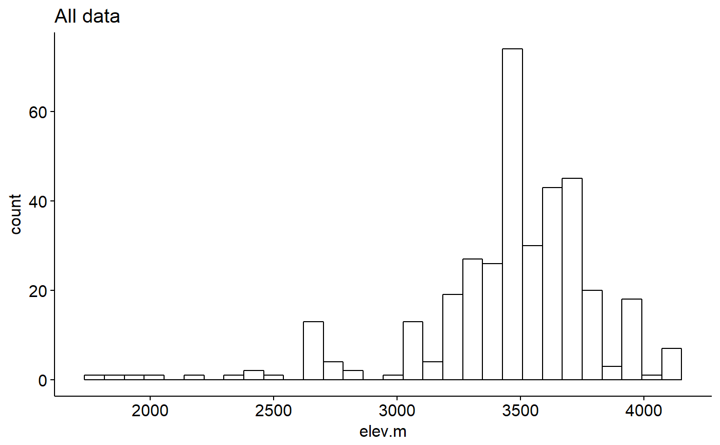
- elev.m
Elevation of site
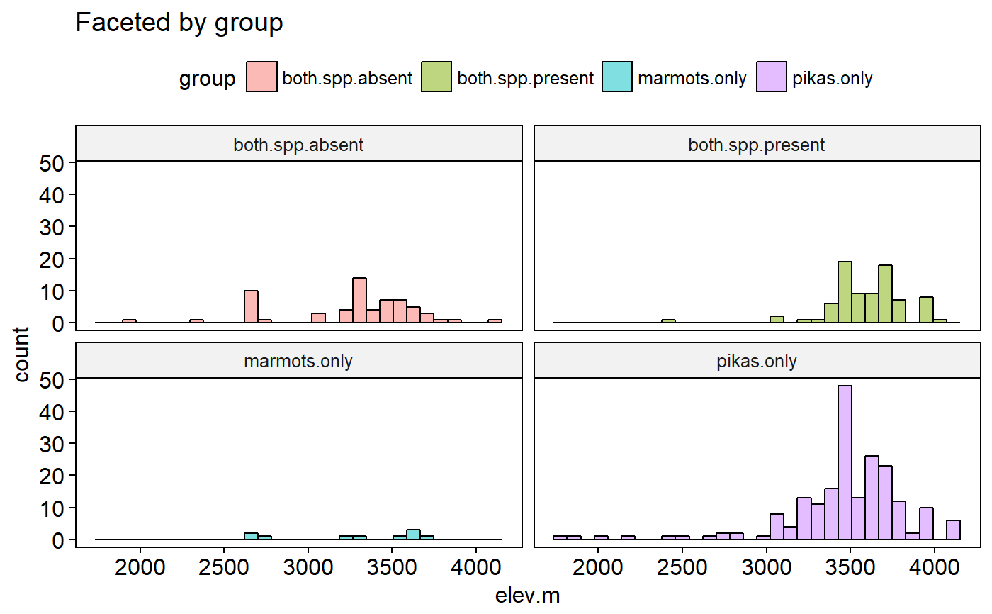
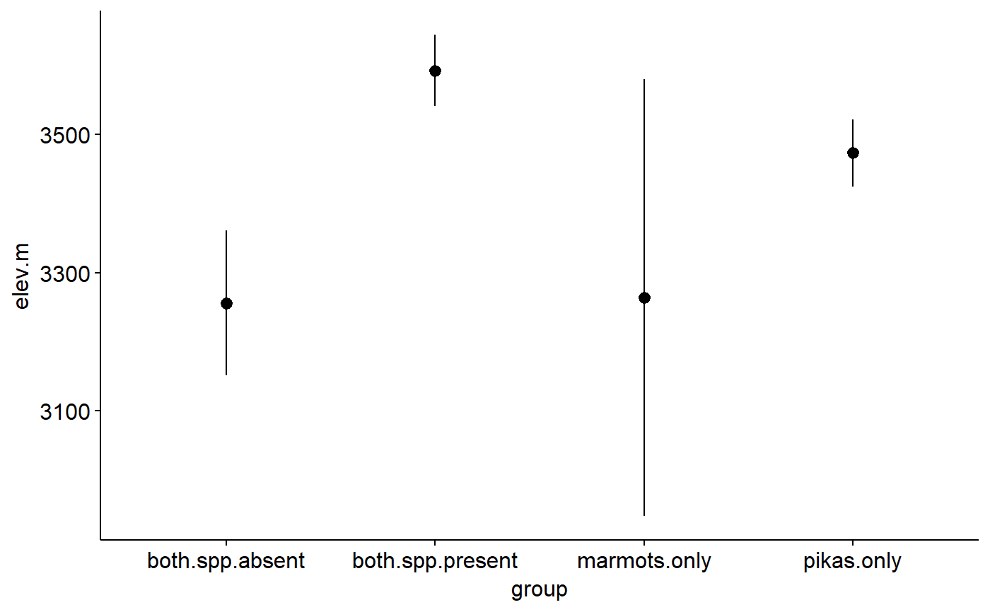
- group
Designates whether no focal species seen, pikas only, marmots only, or both
References
Front Range Pika Project. http://www.pikapartners.org/cwis438/websites/FRPP/Home.php?WebSiteID=18
Examples
## Load packages library(ggplot2) library(ggpubr) ## Explore data graphically ### Plot boxplots ggboxplot(data = pikas, y = "elev.m", x = "group", fill = "group")#> Warning: Using `bins = 30` by default. Pick better value with the argument `bins`.gghistogram(data = pikas, x = "elev.m", facet.by = "group", fill = "group", title = "Faceted by group")#> Warning: Using `bins = 30` by default. Pick better value with the argument `bins`.## Plot means with 95% confidence intervals ggerrorplot(pikas, x = "group", y = "elev.m", desc_stat = "mean_ci", add = "mean")## 1-way ANOVA ### null model model.null <- lm(elev.m ~ 1, data = pikas) ### model of interest model.alt <- lm(elev.m ~ group, data = pikas) ### compare models anova(model.null, model.alt)#> Analysis of Variance Table #> #> Model 1: elev.m ~ 1 #> Model 2: elev.m ~ group #> Res.Df RSS Df Sum of Sq F Pr(>F) #> 1 358 46652447 #> 2 355 42172546 3 4479901 12.57 7.903e-08 *** #> --- #> Signif. codes: 0 '***' 0.001 '**' 0.01 '*' 0.05 '.' 0.1 ' ' 1## Pairwise comparisons after 1-way ANOVA ### no corrections for multiple comparisons pairwise.t.test(x = pikas$elev.m, g = pikas$group, p.adjust.method = "none")#> #> Pairwise comparisons using t tests with pooled SD #> #> data: pikas$elev.m and pikas$group #> #> both.spp.absent both.spp.present marmots.only #> both.spp.present 1.2e-08 - - #> marmots.only 0.9469 0.0047 - #> pikas.only 1.6e-05 0.0084 0.0616 #> #> P value adjustment method: none### Bonferonni correction pairwise.t.test(x = pikas$elev.m, g = pikas$group, p.adjust.method = "bonferroni")#> #> Pairwise comparisons using t tests with pooled SD #> #> data: pikas$elev.m and pikas$group #> #> both.spp.absent both.spp.present marmots.only #> both.spp.present 7.5e-08 - - #> marmots.only 1.000 0.028 - #> pikas.only 9.8e-05 0.050 0.370 #> #> P value adjustment method: bonferroni## Tukey test ### re-fit model with aov() model.alt.aov <- aov(elev.m ~ group, data = pikas) ### TukeyHSD() on model from aov() TukeyHSD(model.alt.aov)#> Tukey multiple comparisons of means #> 95% family-wise confidence level #> #> Fit: aov(formula = elev.m ~ group, data = pikas) #> #> $group #> diff lwr upr p adj #> both.spp.present-both.spp.absent 336.628875 187.57748 485.680266 0.0000001 #> marmots.only-both.spp.absent 7.815778 -295.02921 310.660764 0.9998938 #> pikas.only-both.spp.absent 217.136993 88.90408 345.369906 0.0000956 #> marmots.only-both.spp.present -328.813098 -626.81307 -30.813127 0.0239624 #> pikas.only-both.spp.present -119.491882 -235.82148 -3.162281 0.0415090 #> pikas.only-marmots.only 209.321216 -78.83038 497.472816 0.2406440 #>