Data on the size of Trillium from several sites in Crawford County, PA

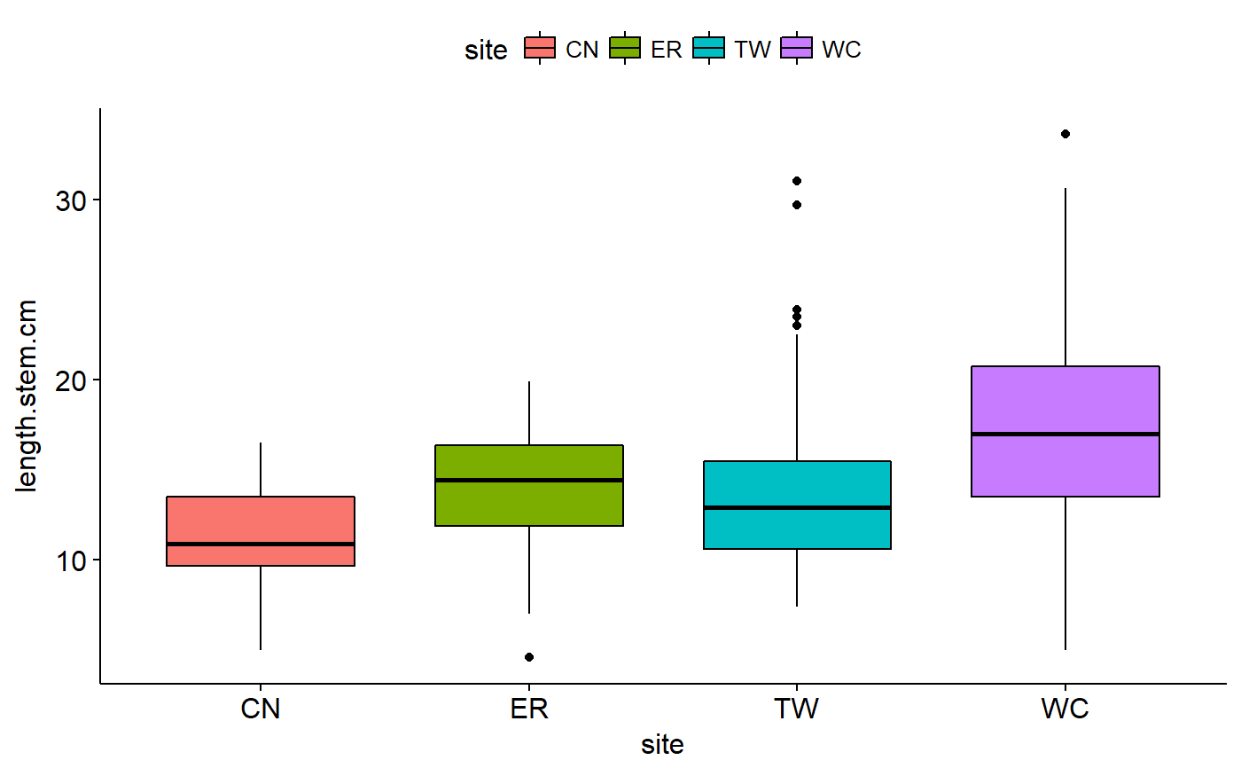
The size of Trillium has been hypothesized to be correlated with the intensity of deer browse occuring on thee population.

trillium

Format

A data frame

site

site code for different forests and woodlots in NW Pennsylvania near the Pymatuning Laboratory of Ecology

spp

species. All are = T for Trillium

length.stem.cm

length from soil to leaf whorl

length.leaf.cm

length of longest leaf in cm

References

Author year.

Examples

library(ggplot2)
library(ggpubr)

## Explore data graphically

### Plot boxplots
ggboxplot(data = trillium,
          y = "length.stem.cm",
          x = "site",
          fill = "site")
#> Warning: Removed 45 rows containing non-finite values (stat_boxplot).

### Plot histograms
gghistogram(data = trillium,
          x = "length.stem.cm",
          title = "All data")
#> Warning: Using `bins = 30` by default. Pick better value with the argument `bins`.
#> Warning: Removed 45 rows containing non-finite values (stat_bin).

 gghistogram(data = trillium,
          x = "length.stem.cm",
          facet.by = "site",
          fill = "site",
          title = "Faceted by site")
#> Warning: Using `bins = 30` by default. Pick better value with the argument `bins`.
#> Warning: Removed 45 rows containing non-finite values (stat_bin).

## Plot means with 95% confidence intervals
ggerrorplot(trillium,
  x = "site",
  y = "length.stem.cm",
  desc_stat = "mean_ci",
  add = "mean")
#> Warning: Removed 45 rows containing non-finite values (stat_summary).
#> Warning: Removed 45 rows containing non-finite values (stat_summary).

## 1-way ANOVA to compare sites

### null model
model.null <- lm(length.stem.cm ~ 1, data = trillium)

### model of interest
model.alt <- lm(length.stem.cm ~ site, data = trillium)

### compare models
anova(model.null, model.alt)
#> Analysis of Variance Table
#> 
#> Model 1: length.stem.cm ~ 1
#> Model 2: length.stem.cm ~ site
#>   Res.Df   RSS Df Sum of Sq      F    Pr(>F)    
#> 1    550 12639                                  
#> 2    547 10012  3    2626.9 47.839 < 2.2e-16 ***
#> ---
#> Signif. codes:  0 '***' 0.001 '**' 0.01 '*' 0.05 '.' 0.1 ' ' 1

## Pairwise comparisons after 1-way ANOVA
### no corrections for multiple comparisons
pairwise.t.test(x = trillium$length.stem.cm, g = trillium$site,
      p.adjust.method = "none")
#> 
#> 	Pairwise comparisons using t tests with pooled SD 
#> 
#> data:  trillium$length.stem.cm and trillium$site 
#> 
#>    CN      ER      TW     
#> ER 0.0036  -       -      
#> TW 0.0046  0.4113  -      
#> WC 2.4e-16 4.0e-08 < 2e-16
#> 
#> P value adjustment method: none 

### Bonferonni correction
pairwise.t.test(x = trillium$length.stem.cm, g = trillium$site,
      p.adjust.method = "bonferroni")
#> 
#> 	Pairwise comparisons using t tests with pooled SD 
#> 
#> data:  trillium$length.stem.cm and trillium$site 
#> 
#>    CN      ER      TW     
#> ER 0.022   -       -      
#> TW 0.028   1.000   -      
#> WC 1.5e-15 2.4e-07 < 2e-16
#> 
#> P value adjustment method: bonferroni 

## Tukey test

### re-fit model with aov()
model.alt.aov <- aov(length.stem.cm ~ site, data = trillium)

### TukeyHSD() on model from aov()
TukeyHSD(model.alt.aov)
#>   Tukey multiple comparisons of means
#>     95% family-wise confidence level
#> 
#> Fit: aov(formula = length.stem.cm ~ site, data = trillium)
#> 
#> $site
#>             diff        lwr      upr     p adj
#> ER-CN  2.6061111  0.3061946 4.906028 0.0190462
#> TW-CN  2.0765353  0.1942317 3.958839 0.0239234
#> WC-CN  6.2315741  4.3338279 8.129320 0.0000000
#> TW-ER -0.5295758 -2.1894709 1.130319 0.8439879
#> WC-ER  3.6254630  1.9480765 5.302849 0.0000002
#> WC-TW  4.1550388  3.1220450 5.188033 0.0000000
#> 

### Plot effect sizes
plotTukeysHSD(TukeyHSD(model.alt.aov))
#> Error in plotTukeysHSD(TukeyHSD(model.alt.aov)): object 'x.values' not found