Chapter 5 The layout of RStudio
To move forward with this book you need to get access to R. There are several ways to do this, and if you are participating in a class your instructor may have a favored way to do it.
5.1 RStudio (Desktop or Cloud)
There are two primary ways to use R relevant to this book:
- Create an account at RStudio Cloud. This is the easiest way to get started; you get 15 hours per month free which is enough for you to get your bearings. Complete instructions for doing this are available in the appendices. Note that RStudio Cloud and RStudio are essentially identical and so all instructions related to RStudio are relevant to RStudio cloud.
- Download R AND RStudio desktop. Key here is that you need TWO pieces of software, R and RStudio. Complete instructions are in the appendices.
These two methods are essentially equivalent. To jump in and get started I recommend RStudio cloud. See the appendices for step by step instructions.
5.2 R emulators
There are also two other ways of using R which we’ll occasionally use. I mention them here briefly. They essentially emulate the R experience but eliminate the hairy details.
- Shiny Apps: These are independent mini-programs that allow you to explore or carryout some aspect of R functionality without doing any coding. They typically live on the internet, but can also be brought up from RStudio desktop. An example of a simple Shiny App on the internet is here: https://shiny.rstudio.com/gallery/faithful.html.
- learnr tutorials: These are interactive tutorials where you do basic coding in your web browser. Here’s an example: https://learnr-examples.shinyapps.io/ex-data-filter/
5.3 Other ways
Two other ways you may encounter R
- Use a Jupyter notebook: Jupyter notebooks are an advanced R emulator. They are really cool, allowing you to essentially combine text (like a tutorial) with code that can be run within a web browser.
- Use regular old R: When you download R an icon will appear on your desktop. You can access old-school R that way, but almost no one ever does. For a bit more information about this see the appendix.
5.4 RStudio at a glance
Now we’ll get started with RStudio. We’ll get to know what it looks like and configure it a bit for out needs.
If you are using RStudio desktop the RStudio logo looks like this:
(#fig:rstudio.logo)The RStudio logo
Whether on the Cloud or Desktop, when you open up you’ll be greeted by a fairly busy array of menus and things. Don’t panic! A typical fresh starting point in RStudio/RStudio Cloud is shown in Figure 2.
(#fig:rstudio.open)RStudio when first opened.
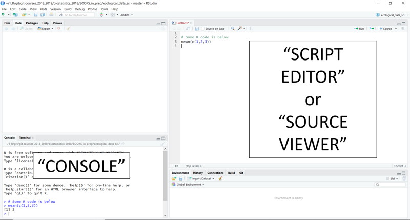
When referring to RStudio (and equivalently RSTudio Cloud - this is the last time I’ll mention this so hopefully get get the point), there are two terms that need to be understood. As shown in Figure 3, there is 1)the console section of RStudio and 2) the script editor or source viewer.

(#fig:rstudio.console)RStudio’s console and script editor.
(A “cheat sheet” called the “RStudio IDE Cheat Sheet” details all of RStudio’s many features and is available at https://www.rstudio.com/resources/cheatsheets/ . It very thorough, though a bit dense. I don’t recommend it for beginners but you should remember that it exists.)
5.4.1 The console versus the script editor
You can type and enter text into both the console and the script editor (also called the source viewer. The console, however, responds actively like a calculator, while the script editor works more like a text editor. Information can be passes unidirectionally from the script editor to the console, but not the other way.
5.4.1.1 The R console
The console in RStudio gives you interactive programming environment that is very similar to a scientific calculator. If you click your mouse inside the console and type 1 + 1 then press enter you will see the following type of output
1 + 1## [1] 2Note that right in front of where you typed 1+1 there is a > symbol. This is always in the R console and never needs to be typed. You may occasionally see it printed in books or on websites, but it doesn’t ever need to be typed.
One thing to note about R is that it’s not particular about spacing. All of the following things will yield the same results
1+1
1 + 1
1          +        1
1 +                                   1
Got it? Awesome! Now we’re ready for some real data analysis.