Chapter 33 The different faces of R code: The console, scripts & RMarkdown
To Do: Change example - currently focuses on t-test using Welch’s correction There are a number of ways to interact with R
- Directly in the console, like a scientific calculator
- Using script files (.R) with
- R code types out and sent over to the console
- notes “commented out” using hashtags “#”
- rmarkdown (.Rmd) files with
- R code in species code chunks
- notes written like in a word processor
- formatting using markdown, a markup language
This chapter will briefly introduce these different ways of working in R
33.1 The console
In a previous chapter we introduced the console. You can interact with the console in a similar manner as a scientific calculator.
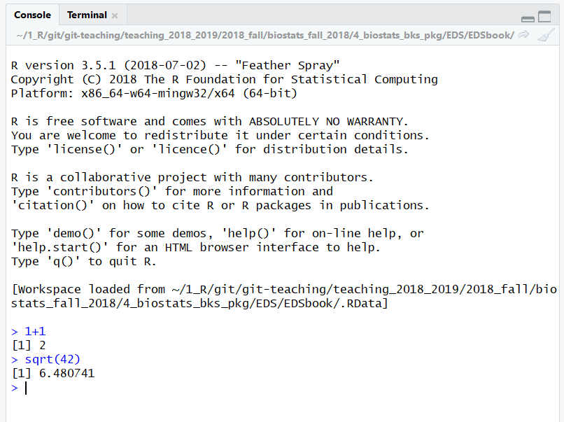
(#fig:first.chnk.sxn1ch4)The RStudio console
As you execute more commands, they move up the screen. You can scroll back up to see what you’ve done previously.
33.2 Scripts
You can create a record of the commands you have executed in the console by copying and pasting or by downloading a log file RStudio creates, but these aren’t very efficient ways to work. If you want to keep track of the commands you’re running (and often you do) its best to write them in a script file and then send them over to the console to execute the code.
33.2.1 Creating scripts
When you open RStudio a blank script file will be open. Subsequently, RStudio will open files you have worked with previously. To create a new blank script file:
- Click on File
- New File
- R script
or just type control + shift + N (on a PC) or command + shift + N on (Mac), which is similar how you make a new document in most programs.
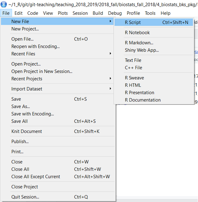
Figure 33.1: Creating a new R script file
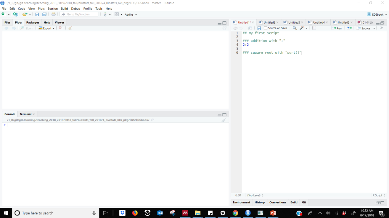
Figure 33.2: R Script file with comments in RStudio
33.2.2 Running code from a script
To run a code you can either place click to the right of the line of code and click the “run” button.
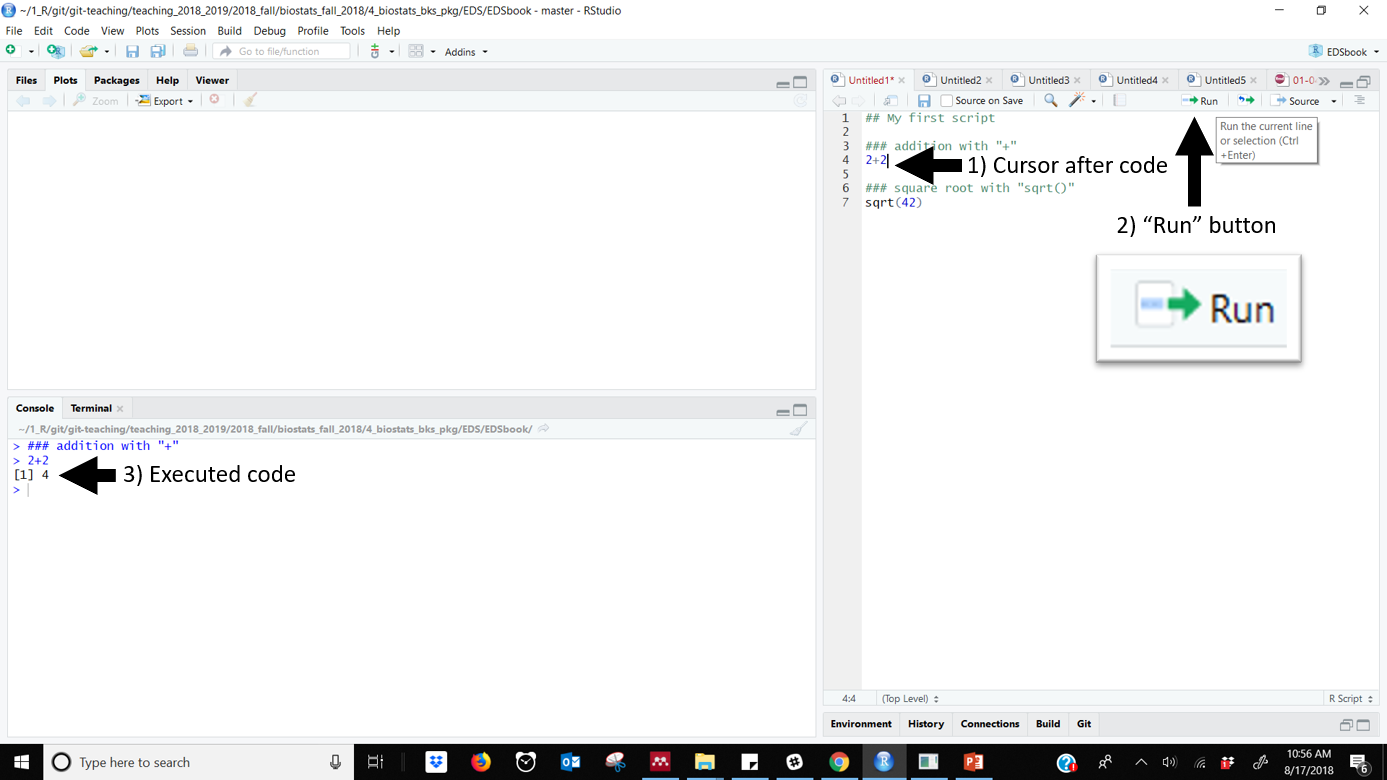
Figure 33.3: Running code using RStudios RUN button. Note cursor to the right of the code
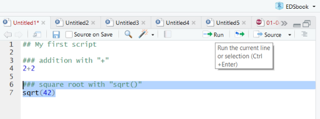
Figure 33.4: Highlighted code in an RStudio script
33.2.3 Running code with keyboard shortcuts
Want to look like an R pro? Learn keyboard shortcuts so you don’t have to use the mouse. Both of the above methods work using simple keyboard shortcuts:
- PCs: Control + Enter
- Macs: Command + Enter
Another handy shortcut is “Control + 2”, which moves your computer’s cursor from the script editor to the console. (Control + 2 moves it from console to editor)
33.3 Organizing scripts
“You mostly collaborate with yourself, and me-from-two-months-ago never responds to email.” (Karen Cranston, paraphrasing Mark Holder; quoted by Megan Duffy on dynamicecology)
Script files perform a record of your work so you can
- remember what you did
- re-run it to check things
- re-use your code for new analyses
- track down errors (which will happen!)
- share with collaborators
Script files are not unique to R, but the R community seems to have built up a particularly good infrastructure for their implementation and ethos encouraging their use. Megan Duffey at Dynamic Ecology has an excellent post on this.
When you first start out learning R most of your scripts will be disposable. Quickly you’ll want to start keeping track of the code you write in class to refer back to. When you start doing analyses you’ll want to write comments as you go, and provide details at the top of your file so you can quickly get up to speed when you come back to the file.
33.3.1 What to include in a script
A good R script should be a self-sufficient document that your future self can easily make sense of, or better yet, someone starting from scratch can understand. Depending on the exact purpose, things to include might be
- A general title, such as “R Script: data exploration &t-test for analysis of frog arm girth”
- Who wrote it and their contact info
- When the script was created
- when it was most recently accessed or created
- What data it uses and where it comes from
- What project or paper it relates to
A challenge when writing and maintaining R scripts is that you are often actively engaged in learning R, learning stats, and learning about or exploring your data. So you write a lot of code then erase it, or scratch out code in a script and then move on. While I have written and saved many scripts that I have never re-opened, I have never re-opened a script and said “wow, I went WAY overboard annotating this thing!” ALso, commenting code makes it much easier to read; I often add fairly simple comments to make code easier navigate and to break things up into smaller chunks.
So, at a minimum I think every script should
- Have some kind of header saying what it is and when it was made
- Have one line of comments or annotations for every 3 to 5 lines of code.
33.3.2 Formatting sections in R scripts
To make scripts easier to navigate its useful to strong together the comment character “#” to make dividers and boxes. This is very good practice to make code more readable. It can be a bit tedious at times to do this; one advantage of rmarkdown, which we’ll introduce at the end of this chapter and go into further in the next, is that it makes it very easy to format section titles.
33.3.3 A sample R script
On the following pages are examples of R scripts for a formal analysis of a dataset. First I’ll show what the script might look like as I write it. Then I’ll show how I’ll fix it up once I know its something I am going to look back at in the future.
### R Script: Analysis of frog arm girth

## Nathan Brouwer (brouwern@gmail.com)
## 6/6/2018
## update: 8/17/2018

## I am re-running analysis from paper by Buzatto  et al 2015
## I want to compare the results of a t-test with
## and w/o Welch's correction for unequal variation

## Packages
library(wildlifeR)

## Data set up
# load frogarm data from Buzatto et al 2015
data("frogarms")


## Data visualization
# histogram of all data
hist(frogarms$sv.length)
## Data analysis
# unpaired t-test NOT using Welch's correction
## NOTE: assumes variation within each group EQUAL
t.test(sv.length ~ sex, # model formula
var.equal = TRUE, # set variances to equal
data = frogarms) # data
# unpaired t-test >>using<< Welch's correction
t.test(sv.length ~ sex,
var.equal = FALSE, # set variances to be unequal
data = frogarms)33.3.4 A polished R script
###########################################
###
### R Script: Analysis of frog arm girth
###
###########################################

## Author:      Nathan Brouwer (brouwern@gmail.com)
## Creation:    6/6/2018
## Last update: 8/17/2018


###############
## Introduction
###############

# This script is an analysis of frog body size and arm girth

## I am re-running analysis from paper by Buzatto  et al 2015
## I want to compare the results of a t-test with
## and w/o Welch's correction for unequal variation
# Data were originally from
# Buzatto et al 2015. Sperm competition and the evolution of
# precopulatory weapons: Increasing male density promotes
# sperm competition and reduces selection on arm strength in
# a chorusing frog. Evolution 69: 2613-2624.
# https://doi.org/10.1111/evo.12766
# Data originally downloaded on 6/6/2018 from
# https://figshare.com/articles/Data_Paper_Data_Paper/3554424
# Data are included in the wildlifeR package and load from it
# https://github.com/brouwern/wildlifeR###############
## Packages
###############
library(wildlifeR)
###############
## Data set up
###############
# load frogarm data from Buzatto et al 2015
data("frogarms")
######################
## Data visualization
######################
# histogram of all data
hist(frogarms$sv.length)######################
## Data analysis
######################
# unpaired t-test NOT using Welch's correction
## NOTE: assumes variation within each group EQUAL
t.test(sv.length ~ sex, # model formula
var.equal = TRUE, # set variances to equal
data = frogarms) # data
# unpaired t-test >>using<< Welch's correction
t.test(sv.length ~ sex,
var.equal = FALSE, # set variances to be unequal
data = frogarms)For more on organizing scripts see points 4 and 5 of “Eight things I do to make my open research more findable and understandable” at (DataColada](http://datacolada.org/69).