<ol start="6" style="list-style-type: lower-alpha"> <li>Analysis walthrough: t-test and friends</li> </ol> • shroom

Introduction

This tutorial walks through several types of anlayses that can be done using the shroom package. The focus will be on situations that can be analyzed using t-tests and similar methods to compare 2 groups. In particular

Testing for groups differences using a t-test (t.test)
Cohen’s d effect size for the differene between 2 means (effsizeeffsize:cohen.d)
Formulating a t-test as a linear model (lm)
Non-parametric test for ranked data (wilcox.test)
Non-parametric for skewed rank data (lawstat::brunner.munzel.test)

TO DO

Things not yet implemented

for Welch-type tests
effect size calculations with metafor
effect size for non-parametric tests

Preliminaries

Load packages

Load the shroom package. You can download it with instal.packages(“shroom”) if you haven’t used it ever before. See “Loading the shroom package” for more information.

library(shroom)

Load other essential packages

library(ggpubr)  #plotting
#> Loading required package: ggplot2
#> Loading required package: magrittr
library(cowplot)
#> 
#> Attaching package: 'cowplot'
#> The following object is masked from 'package:ggpubr':
#> 
#>     get_legend
#> The following object is masked from 'package:ggplot2':
#> 
#>     ggsave

library(dplyr)   #data cleaning
#> 
#> Attaching package: 'dplyr'
#> The following objects are masked from 'package:stats':
#> 
#>     filter, lag
#> The following objects are masked from 'package:base':
#> 
#>     intersect, setdiff, setequal, union

    library(car)     #?
#> Loading required package: carData
#> 
#> Attaching package: 'car'
#> The following object is masked from 'package:dplyr':
#> 
#>     recode

    library(data.tree)# plotting data structure
    library(treemap)

library(plotrix) #std.err function

library(bbmle)   #AIC table
#> Loading required package: stats4
#> 
#> Attaching package: 'bbmle'
#> The following object is masked from 'package:dplyr':
#> 
#>     slice
library(lme4)
#> Loading required package: Matrix
library(lawstat) #?
#> Loading required package: Kendall
#> Loading required package: mvtnorm
#> Loading required package: VGAM
#> Loading required package: splines
#> 
#> Attaching package: 'VGAM'
#> The following object is masked from 'package:bbmle':
#> 
#>     AICc
#> The following object is masked from 'package:car':
#> 
#>     logit
#> 
#> Attaching package: 'lawstat'
#> The following object is masked from 'package:car':
#> 
#>     levene.test
library(effsize) #Cohen's dw

Load data

Loading data directly from the shroom package

The data are internal to the package and so can be easily loaded.

data("wingscores")

Loading the data from the shroom package

For a real analysis you need to start from the .csv file with the raw data, eg data_ind_flies_expt1_2018.csv if you are working with the 2018 shroom data. This data is included when you download the package. If you search your computer for it you should be able to locate it. It is in a diretory called “extdata” within the directory for the shroom package which you downloaded.

Save the file data_ind_flies_expt1_2018.csv to where you want to do your work for this project
Set your working directory to the same folder where the file is saved. This can be done through “Session” option of the RStudio menu (this will occur automatically if you are using an R project).
Load the data using read.csv OR the “Import Dataset” button within RStudio

Using the “Import Dataset” button is helpful because it brings up a file navigation system that is similar to a normal program and generates the code you need to load the data.

Its good to copy and paste this code into your script so you always have it.

Note that the code generated by “Import Dataset” creates an absolute path for the file name. This means that if you move the file that the original code will no longer work and you will have to got back through the “Import Dataset” process again.

Adanced: Loading data using relative file paths

Because I am familiar with the ins and outs of R I use “relative file paths”; if I move files, my code accomodates them being moved. However, this is a bit abstract and is more advanced. You are encouraged to skip this section if you are new to R.

There here() fuction of there here packages tells me where an RStudio project file is.

here::here()
#> [1] "C:/Users/lisanjie/Documents/shroom_master/shroom"

I can construct a valid, flexible flie path using here::here()

# You don't need to do this
path. <- here::here("inst/extdata")

What is in the directory

list.files(path.)
#> [1] "data_ind_fly_wing_scores_2018.csv"

Full file path

file. <- here::here("inst/extdata/data_ind_fly_wing_scores_2018.csv")

I then load the data

# load data using path and file saved in file. object
flies <- read.csv(file.)

Cleaning and subsetting the wing data

This information is covered in more detail in “Subsetting a dataframe with dplyr.”

Examine raw data

dim(flies)
#> [1] 7754   16
names(flies)
#>  [1] "student.ID"  "seat"        "gene"        "allele"      "section"    
#>  [6] "file"        "loaded"      "E.or.C"      "sex"         "group"      
#> [11] "wing.score"  "stock.num"   "temp.C"      "allele.num"  "gene.shrt"  
#> [16] "gene.allele"
head(flies)
#>   student.ID seat gene allele section         file loaded E.or.C sex group
#> 1          1    1  abl abl[2]    AM.M wing_01.xlsm loaded      E   M   E.M
#> 2          1    1  abl abl[2]    AM.M wing_01.xlsm loaded      E   M   E.M
#> 3          1    1  abl abl[2]    AM.M wing_01.xlsm loaded      E   M   E.M
#> 4          1    1  abl abl[2]    AM.M wing_01.xlsm loaded      E   M   E.M
#> 5          1    1  abl abl[2]    AM.M wing_01.xlsm loaded      E   M   E.M
#> 6          1    1  abl abl[2]    AM.M wing_01.xlsm loaded      E   M   E.M
#>   wing.score stock.num temp.C allele.num gene.shrt gene.allele
#> 1          5      8565     25          1       abl       abl.1
#> 2          5      8565     25          1       abl       abl.1
#> 3          5      8565     25          1       abl       abl.1
#> 4          5      8565     25          1       abl       abl.1
#> 5          5      8565     25          1       abl       abl.1
#> 6          5      8565     25          1       abl       abl.1

Clean the raw data

Remove some un-needed columns using select().
Note “-” before each column name.

flies <- flies %>% select(-stock.num,
                          -loaded,
                          -file,
                          -gene,
                          -temp.C)

Data frame now has fewer columns

dim(flies)
#> [1] 7754   11

Data analysis

We will walk through analyses comparing just two groups: female control flies versus female experimental flies. In subsequent tutorials we’ll look at more complex data.

Nomeclature: “Student”" vs. “fly-level”" data

Because these data result from summarizing the work done by each student, I will refer to it as student-level data. In contrast, the raw data generated by the student is fly-level data because each data point represents a single fly.

Data from 1 student: t-test

Extract data for a single student using the dplyr::filter() command.
Select on TWO conditions: student.ID == 1 AND sex == “F”

student1.F <- flies %>% filter(student.ID ==  1 &
                                    sex == "F")

Data frame now has many fewer rows

dim(student1.F)
#> [1] 24 11

Data exploration

Examine the data and consider the issues raised by Consider the issues raied by Zuur et al 2010

Structure of the data

We can think of the data like this

working <- student1.F
working$i <- 1:nrow(working)

i.E <- which(working$E.or.C == "E")

i.use <- c(min(working$i[i.E])
,min(working$i[i.E])+1
,max(working$i[i.E])-1
,max(working$i[i.E])
,min(working$i[-i.E])
,min(working$i[-i.E])+1
,max(working$i[-i.E])-1
,max(working$i[-i.E]))

i.medians <- round(c(median(working$i[i.E])
,median(working$i[-i.E])),0)



working[-i.use, "i"] <- "*\n*\n*"



working$pathString <- with(working,
                              paste(allele,
                                    E.or.C,
                                    i,
                                    sep = "/"))

i <- sort(c(i.use,i.medians))
working.tree <- as.Node(working[i,])

SetGraphStyle(working.tree,
              rankdir="LR")

plot(working.tree)

Plot histogram using ggpubr::gghistogram

Is data normal?
is data skewed?
Is variance constant between groups?

gghistogram(data = student1.F,
            x = "wing.score",
            fill = "E.or.C", 
            add = "mean",       #add line formean
            position = "dodge") #
#> Warning: Using `bins = 30` by default. Pick better value with the argument
#> `bins`.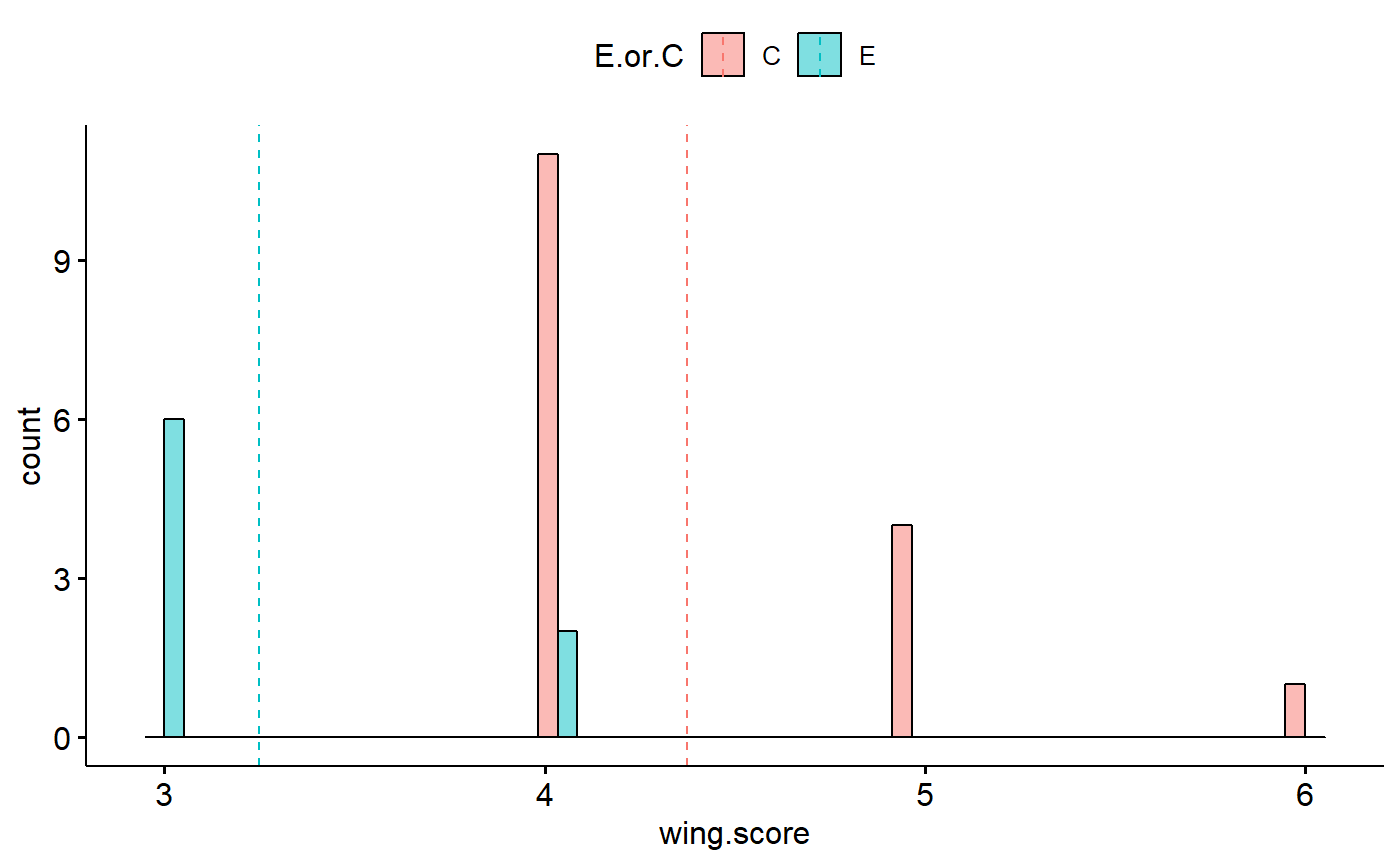

Plot boxplot

Is data normal?
is data skewed?
Is variance of different groups constant?

ggboxplot(data = student1.F,
            y = "wing.score",
            x = "E.or.C",
            add = "mean",
            fill = "E.or.C")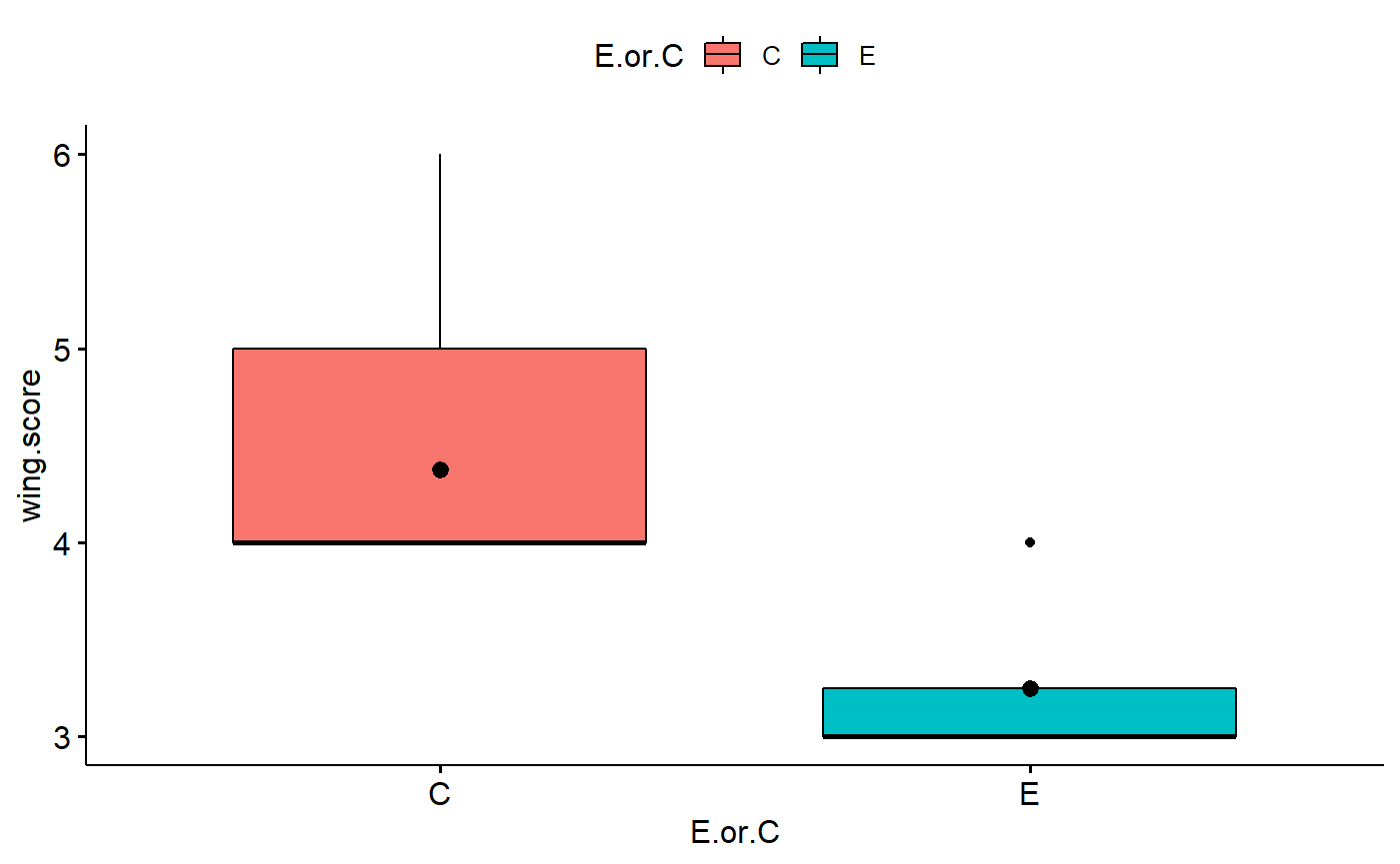

Numeric summaries

Numeric summaries are useful when writing about the results and summarizing them for potential future meta-anlysts.

Step:

group_by(E.or.C) splits into treatments
numeric summaries (mean, sd) called on wing score
note that I can do math within summarize()
std.error function is from plotrix package

student1.F %>% 
  group_by(E.or.C) %>% 
  summarize(mean = mean(wing.score),
            n = n(),
            sd = sd(wing.score),
            se = plotrix::std.error(wing.score),
            CI95 = 1.96*std.error(wing.score))
#> # A tibble: 2 x 6
#>   E.or.C  mean     n    sd    se  CI95
#>   <fct>  <dbl> <int> <dbl> <dbl> <dbl>
#> 1 C       4.38    16 0.619 0.155 0.303
#> 2 E       3.25     8 0.463 0.164 0.321

Data analysis: t-test

Consider these questions after you run the test:

What are the assumptions of the t-test?
Are we violating them?
Which issues does Welch’s t-test solve?
Which issues does it NOT solve?

t.test(wing.score ~ E.or.C, 
       data = student1.F)
#> 
#>  Welch Two Sample t-test
#> 
#> data:  wing.score by E.or.C
#> t = 4.9941, df = 18.293, p-value = 8.977e-05
#> alternative hypothesis: true difference in means is not equal to 0
#> 95 percent confidence interval:
#>  0.6522796 1.5977204
#> sample estimates:
#> mean in group C mean in group E 
#>           4.375           3.250

Cohen’s D effect size

Cohen’s D is an relative effect size measure. It is sometiems called a standardized mean difference (SMD) because it is the difference between the means of two groups, “standardized” by a standard deviation pooled from from the 2 groups: (mean.1 - mean.2)/pooled.SD, where pooled.SD is a “weighted” mean of the two SDs. In meta analysis it is more commone now I think to use a simliar effecti size, Hedge’s g.

Cohen’s d makes all the same assumptions as a t-test BUT does NOT have the ability to correct like Welch’s t-test.

Recent work, including some by ecologists, has shown that in meta-analysis Cohen’s D can become problematic because of issues realted to small sample sizes.
Additinally, I am not sure but I suspect with highly skewed data it is not a good measure of effect, but this is something I want to investigated

effsize::cohen.d(wing.score ~ E.or.C, 
       data = student1.F)
#> 
#> Cohen's d
#> 
#> d estimate: -2.172829 (large)
#> 95 percent confidence interval:
#>       inf       sup 
#> -3.281639 -1.064018

Analysis: T-test as linear regression

Fit 2 models
Note that there is no such thing as a “Welch’s linear model!” so non-constant variance is problematic. This can be corrected using a technique called generlized least squares (gls).

Fit linear models

m.H0 <- lm(wing.score ~ 1,      data = student1.F)
m.Ha <- lm(wing.score ~ E.or.C, data = student1.F)

We can also calcualte a means model by dropping the intercept

m.means <- lm(wing.score ~ -1 + E.or.C, 
              data = student1.F)

Intepret model equation

The model has two paramters

summary(m.Ha)
#> 
#> Call:
#> lm(formula = wing.score ~ E.or.C, data = student1.F)
#> 
#> Residuals:
#>    Min     1Q Median     3Q    Max 
#> -0.375 -0.375 -0.250  0.625  1.625 
#> 
#> Coefficients:
#>             Estimate Std. Error t value Pr(>|t|)    
#> (Intercept)   4.3750     0.1435  30.485  < 2e-16 ***
#> E.or.CE      -1.1250     0.2486  -4.526 0.000167 ***
#> ---
#> Signif. codes:  0 '***' 0.001 '**' 0.01 '*' 0.05 '.' 0.1 ' ' 1
#> 
#> Residual standard error: 0.5741 on 22 degrees of freedom
#> Multiple R-squared:  0.4821, Adjusted R-squared:  0.4586 
#> F-statistic: 20.48 on 1 and 22 DF,  p-value: 0.000167

The general model in R-like notation is wing.score ~ treatment

THis is defined by 2 parameters the intercept and the treatment effect. The treatment effect in this case corresponds to the difference between the two treatments.

The general model with both parameters is: wing.score ~ intercept + treatment.effect

We can plug in the values we have: wing.score ~ 4.8 + -0.63*(Experimental?)

where Experimental? = 0 if its the control treatment and 1 if its the experimental treatment. TWo equations are therefore implied

Control flies: wing.score ~ 4.8 + -0.630 Experimental flies: wing.score ~ 4.8 + -0.631

Which simplfies to

Control flies: wing.score ~ 4.8 Experimental flies: wing.score ~ 4.8 + -0.63

Inference

We can compare the models using p-values or AIC.

Get p-value by comparing models using anova()

anova(m.H0, #null model
      m.Ha) #alternative model
#> Analysis of Variance Table
#> 
#> Model 1: wing.score ~ 1
#> Model 2: wing.score ~ E.or.C
#>   Res.Df   RSS Df Sum of Sq      F   Pr(>F)    
#> 1     23 14.00                                 
#> 2     22  7.25  1      6.75 20.483 0.000167 ***
#> ---
#> Signif. codes:  0 '***' 0.001 '**' 0.01 '*' 0.05 '.' 0.1 ' ' 1

Compare models with AIC. AICtab is from the package bbmle

bbmle::AICtab(m.H0, m.Ha)
#>      dAIC df
#> m.Ha  0.0 3 
#> m.H0 13.8 2

AICc is a better choice than AIC. This requires ICtab()

bbmle::ICtab(m.H0, 
              m.Ha,
             type = "AICc")
#>      dAICc df
#> m.Ha  0.0  3 
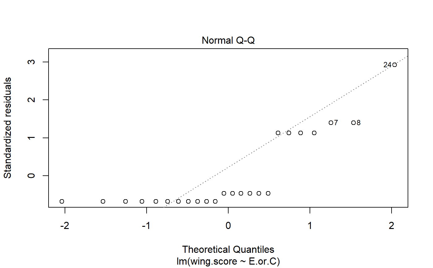
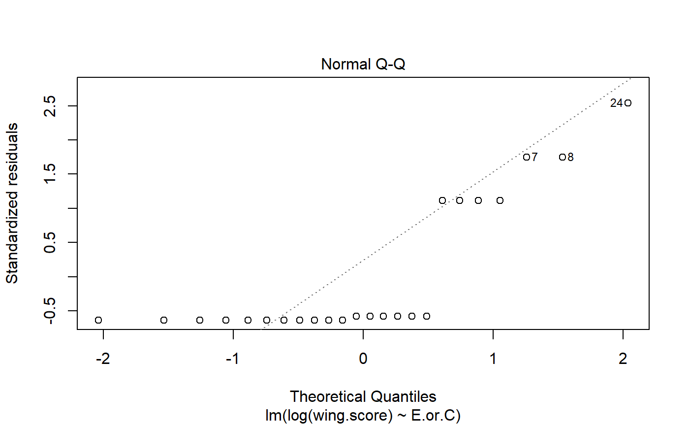
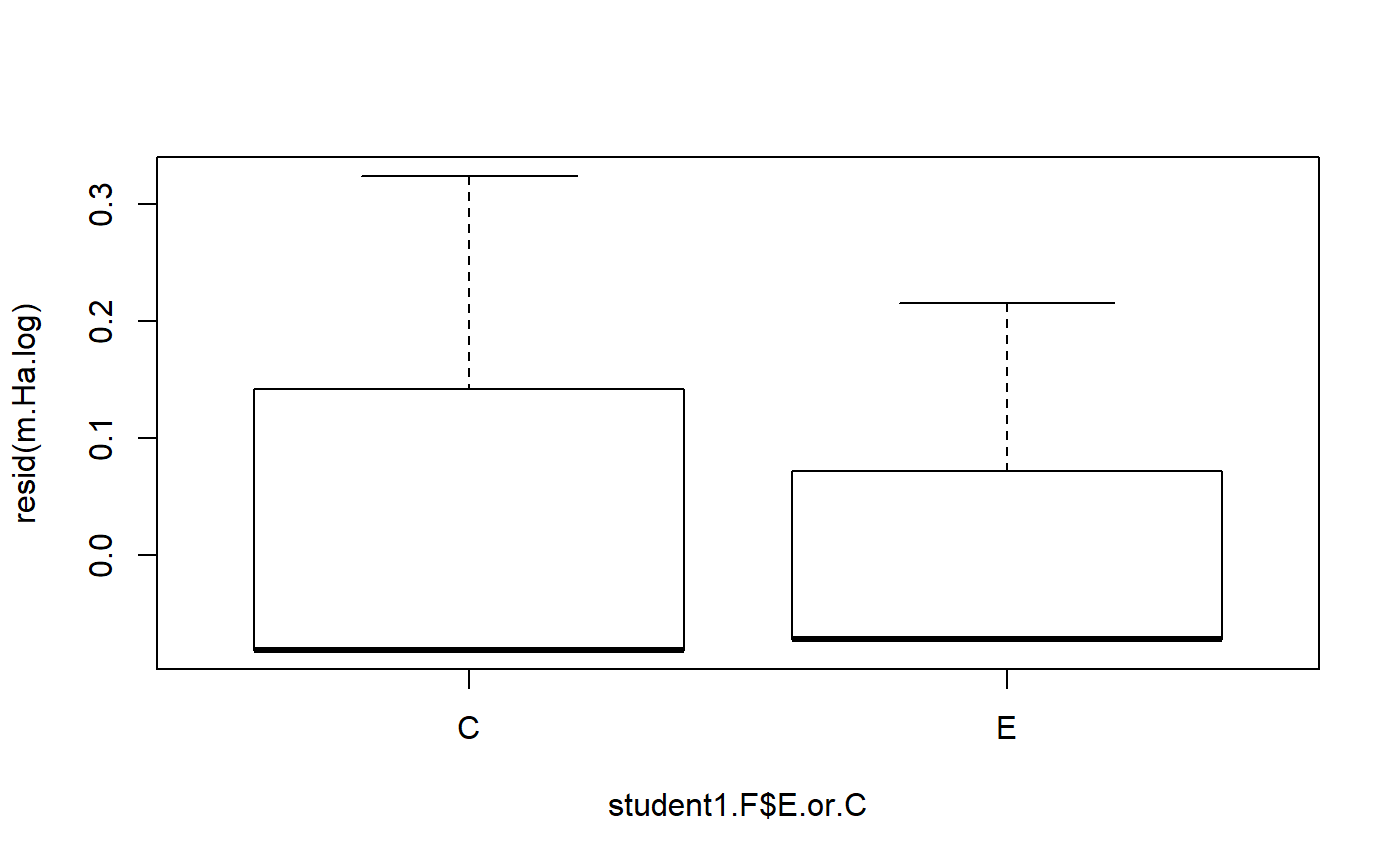
#> m.H0 13.2  2

Model diagnostics

t-test does not provide information on model residuals
lm() does
useful function: resid()

In this context, resid subtracts the group mean (E or C) from each value. This is how much each observation differs from the group mean.

resid(m.Ha)
#>      1      2      3      4      5      6      7      8      9     10 
#> -0.250 -0.250 -0.250 -0.250 -0.250 -0.250  0.750  0.750 -0.375 -0.375 
#>     11     12     13     14     15     16     17     18     19     20 
#> -0.375 -0.375 -0.375 -0.375 -0.375 -0.375 -0.375 -0.375 -0.375  0.625 
#>     21     22     23     24 
#>  0.625  0.625  0.625  1.625

The mean of the residuals is approximately zero

mean(resid(m.Ha))
#> [1] -1.616816e-17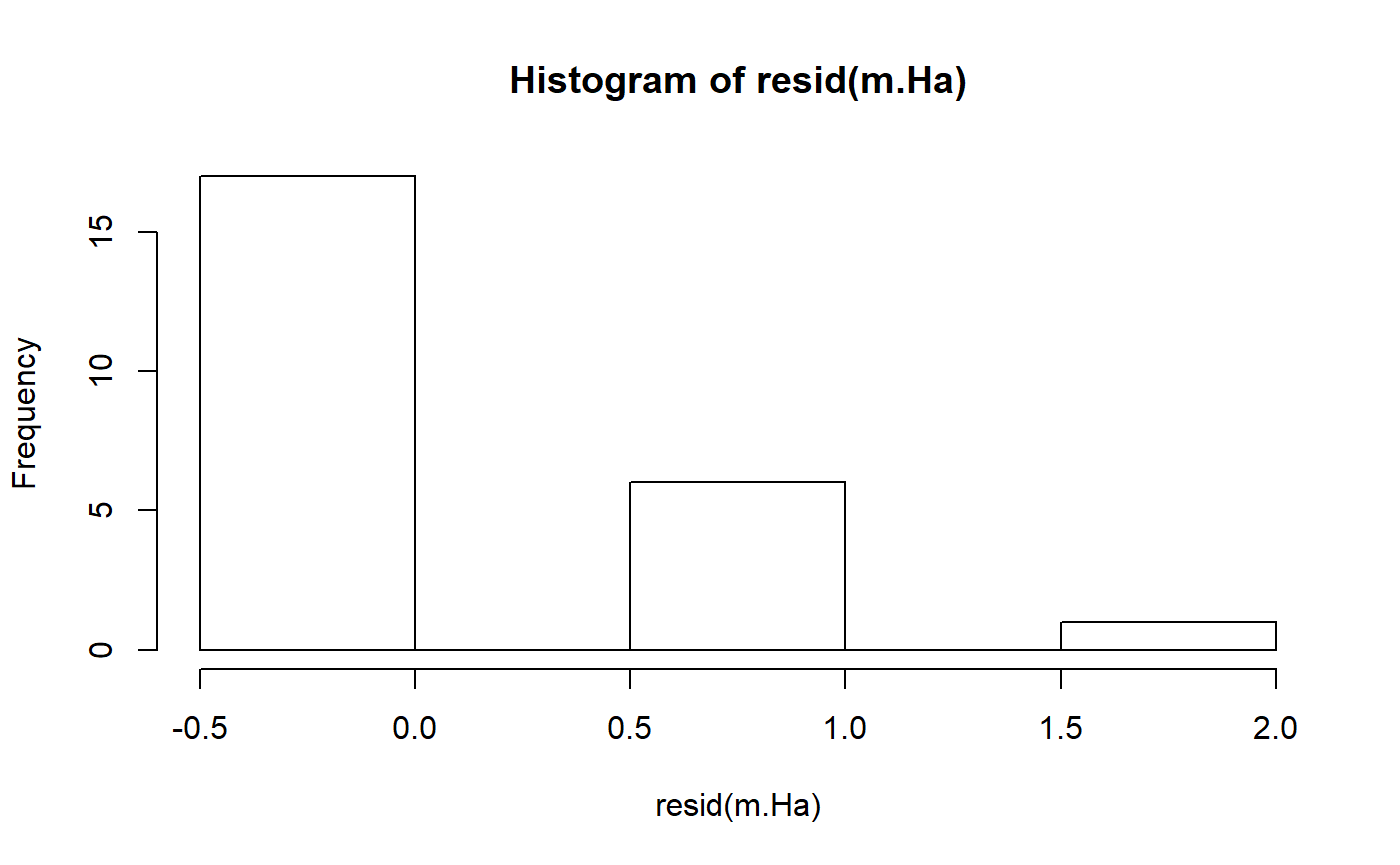

Histogram of residuals

When data are normally distributed within each group, the residuals should be normal…

hist(resid(m.Ha))

Look at normality with a qq-plot

plot(m.Ha, which = 2)

Transformations

Log transformation to improve normality.
Can also help with non-constant variance (heterogenous variance)
log transform is common in regression, and perhaps anova
for some reason people rarely transform t-tests

We can wrap our y variable wing.score in log()

m.H0.log <- lm(log(wing.score) ~ 1, data = student1.F)
m.Ha.log <- lm(log(wing.score) ~ E.or.C, 
               data = student1.F)

Look at p-value for transformed data

P-value is actually lower (not always the case)
Note that log transformation makes subtle changes to how hypotheses are formulated / results interpreted
I am not good at explaining this; some people make a big deal about it; others don’t
will provide references

#raw data
anova(m.H0, 
      m.Ha)
#> Analysis of Variance Table
#> 
#> Model 1: wing.score ~ 1
#> Model 2: wing.score ~ E.or.C
#>   Res.Df   RSS Df Sum of Sq      F   Pr(>F)    
#> 1     23 14.00                                 
#> 2     22  7.25  1      6.75 20.483 0.000167 ***
#> ---
#> Signif. codes:  0 '***' 0.001 '**' 0.01 '*' 0.05 '.' 0.1 ' ' 1

#transformed data
anova(m.H0.log, 
      m.Ha.log)
#> Analysis of Variance Table
#> 
#> Model 1: log(wing.score) ~ 1
#> Model 2: log(wing.score) ~ E.or.C
#>   Res.Df     RSS Df Sum of Sq      F    Pr(>F)    
#> 1     23 0.85251                                  
#> 2     22 0.38241  1    0.4701 27.045 3.247e-05 ***
#> ---
#> Signif. codes:  0 '***' 0.001 '**' 0.01 '*' 0.05 '.' 0.1 ' ' 1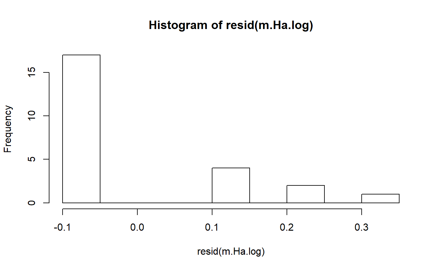

Look at residuals

Histogram of residuals for log transformation

Not much better…

hist(resid(m.Ha.log))

qqplot of residuals for log transformation

More informative that histogram of the residuals; dots should fall on the line…

plot(m.Ha.log,  2)

Look at heteroskedasticity

Plot residuals versus group
Variance still bad…

# column with group variables
summary(student1.F$E.or.C)
#>  C  E 
#> 16  8

#    residuls of model       column with group var
plot(resid(m.Ha.log)    ~    student1.F$E.or.C)

Analysis Non parametric methods

These data are inherently ordina (ordered categories)
Can be thought of as ranks, allowing for ties, with a minimum rank of 1 and a max of 8
Wilcoxon test is the appropriate non-parametic test for ordinal data (also called Mann-Whiteny or Wilcox-Mann-Whitney)
Related terms: Wilcoxon sign-rank test, Mann-Whitney U-test
In the past many people would transform numeric data into ranks if it was highly skewed or otherwise non-normal
This causes a LOT of loss of information and usually reduces statistical power to detect differences between groups when they exist
These data, however, are indeed ordinal/ranks so there is no loss of information content by transformation
A Wilcox test is argueably more appropriate, but people debate this (or are stuck in their ways of doing things)

Run the test

wilcox.test(wing.score ~ E.or.C, 
            data = student1.F)
#> Warning in wilcox.test.default(x = c(4L, 4L, 4L, 4L, 4L, 4L, 4L, 4L, 4L, :
#> cannot compute exact p-value with ties
#> 
#>  Wilcoxon rank sum test with continuity correction
#> 
#> data:  wing.score by E.or.C
#> W = 117, p-value = 0.0003917
#> alternative hypothesis: true location shift is not equal to 0

You might see an error “cannot compute exact p-value with ties.” The computation of the p-values depend on whether there are ties or not in the data; I doubt this is an issue ever in pratice.

Compare p-values: both are very small. The t-test p-value is a bit smaller. Often when you use a test and violate some of its assumptions, your p-values are too big.

wilcox.test(wing.score ~ E.or.C, 
            data = student1.F,
            exact = F)$p.value
#> [1] 0.0003916797
t.test(wing.score ~ E.or.C, 
            data = student1.F)$p.value
#> [1] 8.976852e-05

Wilcox test, normality, and skew

Am just learning about this
Wilcox test does fine with non-normal data…
…except, as I understand it when there is high skew
Wilcox test also doesn’t accomodate non-constant variance
Improved Wilcox test:brunner.munzel.test()

Seperate out each group into seperate object

S1.F.E <- student1.F %>% filter(E.or.C == "E")
S1.F.C <- student1.F %>% filter(E.or.C == "C")

run test

brunner.munzel.test(x = S1.F.E$wing.score,
                    y = S1.F.C$wing.score)
#> 
#>  Brunner-Munzel Test
#> 
#> data:  S1.F.E$wing.score and S1.F.C$wing.score
#> Brunner-Munzel Test Statistic = 7.1127, df = 8.0062, p-value =
#> 0.0001003
#> 95 percent confidence interval:
#>  0.7798382 1.0482868
#> sample estimates:
#> P(X<Y)+.5*P(X=Y) 
#>        0.9140625

Analysis walthrough: t-test and friends

Nathan Brouwer

2018-12-11