Appendix 5) Study Diagrams (REQUIRED image/pptx)
Vignette Author
2018-12-10
Appendix-5-study_diagram.RmdIntroduction
A diagram is often very useful for showing where a study took place, how an experiment was designed, how treatments were allocated, or how there are dependencies in the data. Zuur & Ieno (2016) emphasize this (“Step 2: Visualize the experimental design” and “Step 4: Identify the dependency structure in the data”; see Figure 4).
What follows are references to different types of diagrams that you could include in your study.
Below is also an example using a graph of the hierarchical phylogenetic relationships.
Site maps: Where a study took place
These papers have examples of site maps for ecological studies; both maps are in the supplemental information. The focus in more on providing contextual geographic information than the details of the study.
Latta, Brouwer et al. Avian community characteristics and demographics reveal how conservation value of regenerating tropical dry forest changes with forest age. PeerJ https://peerj.com/articles/5217/#supp-1
Latta, Brouwer et al. Long-term monitoring reveals an avian species credit in secondary forest patches of Costa Rica. PeerJ https://peerj.com/articles/3539/#supplemental-information
Experimental layout maps
Ecological studies sometimes include maps to show the geometric arrangement of study plots or experimental treatments.
Historic disturbance regimes promote tree diversity only under low browsing regimes in eastern deciduous forest T Nuttle, AA Royo, MB Adams… - Ecological Monographs, 2013 - Wiley Online Library
Long-term biological legacies of herbivore density in a landscape‐scale experiment: forest understoreys reflect past deer density treatments for at least 20 years T Nuttle, TE Ristau, AA Royo - Journal of Ecology, 2014
Accounting for multilevel data structures in fisheries data using mixed models T Wagner, DB Hayes, MT Bremigan - Fisheries, 2006
Dependency structure diagrams
For complex experiments it can be useful to create a diagram that illustrate the hierarchical structure of the data, such as students in class rooms in schools in school districts in counties in states.
MCDB / Bio-medicine
Improving basic and translational science by accounting for litter-to-litter variation in animal models SE Lazic, L Essioux - BMC neuroscience, 2013
Four simple ways to increase power without increasing the sample size Stanley E Lazic Laboratory Animals https://journals.sagepub.com/doi/full/10.1177/0023677218767478
Analyzing clustered data: why and how to account for multiple observations nested within a study participant? EL Moen, CJ Fricano-Kugler, BW Luikart, AJ O’Malley - Plos one, 2016
Ecology
Nested by design: model fitting and interpretation in a mixed model era H Schielzeth, S Nakagawa - Methods in Ecology and Evolution, 2013
Meta-evaluation of meta-analysis: ten appraisal questions for biologists S Nakagawa, DWA Noble, AM Senior… - BMC …, 2017 https://bmcbiol.biomedcentral.com/articles/10.1186/s12915-017-0357-7
Nonindependence and sensitivity analyses in ecological and evolutionary meta-analyses …, M Lagisz, RE O’dea, S Nakagawa - Molecular …, 2017
Zuur & Ieno. 2016. A protocol for conducting and presenting results of regression‐type analyses https://besjournals.onlinelibrary.wiley.com/doi/full/10.1111/2041-210X.12577
Graphical abstracts
Graphical abstracts are becoming increasingly common in some fields.
https://www.elsevier.com/authors/journal-authors/graphical-abstract
http://crosstalk.cell.com/blog/attract-readers-at-a-glance-with-your-graphical-abstract
https://bitesizebio.com/31125/how-to-make-a-good-graphical-abstract/
Flow charts
Clinical trials
Clinical trials often have a flow chart showing how an initial patient population was screen and then allocated to the experimental groups.
https://openi.nlm.nih.gov/detailedresult.php?img=PMC2945952_1471-2474-11-205-2&req=4
Meta-analyses
Meta-analyses often have flow charts showing how an initial pool of studies was screen for inclusion in the analysis. The PRISMA guidlines (Preferred Reporting Items for Systematic Reviews & Meta-Analyses) recommend a 4-phase flow diagram be included in meta-analyses to describe the process of finding, screening, and extracting data from papers in a meta analysis. See Libarati et al 2009
I’ve copied an example using You’ll need to install the package if you want to make it yourself eg run install.packages(“PRISMAstatement”). See the PRISMAstatement package for details
library(PRISMAstatement)
prisma(found = 750,
       found_other = 123,
       no_dupes = 776,
       screened = 776,
       screen_exclusions = 13,
       full_text = 763,
       full_text_exclusions = 17,
       qualitative = 746,
       quantitative = 319,
       width = 300, height = 300)
A real example is at https://openi.nlm.nih.gov/detailedresult.php?img=PMC2559819_1471-2261-8-24-1&req=4
Coordinated experiments across labs
The paper below has an interesting flow chart about how samples were shared across three labs to test for biases in lab techniques. The ends result was a retraction of a Cell paper!
Resolving discrepant findings on ANGPTL8 in beta-cell proliferation: a collaborative approach to resolving the betatrophin controversy AR Cox, O Barrandon, EP Cai, JS Rios, J Chavez… - PloS one, 2016
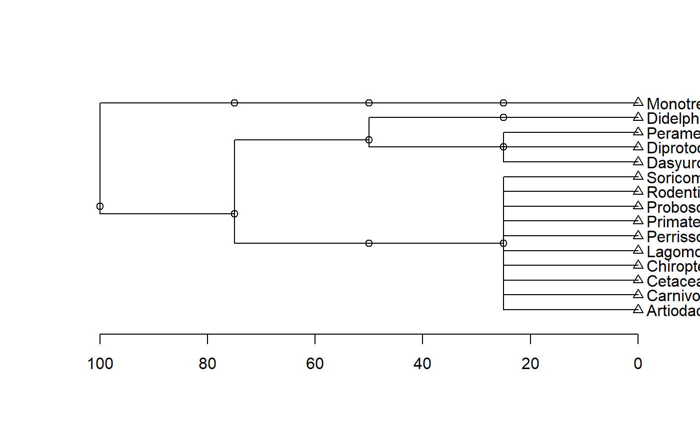
Dependency structure due to phylogeny
The dependency structure in the mammals milk data is due to phylogeny. The original paper presents a phylogenetic tree as a figure. Similarly, code below is a first attempt to visualize this based on nominal taxonomic categories (class, order, family, genus, species). Its not very clean yet.
Conceptual issues of clustering
The following papers discuss conceptual issues of grouping, clustering etc, but don’t have pictures of it.
A solution to dependency: using multilevel analysis to accommodate nested data E Aarts, M Verhage, JV Veenvliet, CV Dolan… - … neuroscience, 2014
What exactly is ’N’in cell culture and animal experiments? SE Lazic, CJ Clarke-Williams, MR Munafò - PLoS biology, 2018
The problem of pseudoreplication in neuroscientific studies: is it affecting your analysis? SE Lazic - BMC neuroscience, 2010
Using biological insight and pragmatism when thinking about pseudoreplication N Colegrave, GD Ruxton - Trends in ecology & evolution, 2017
Visualizing the structure of the mammals milk data
What follows is a code dump to make a diagram of the mammals milk data set. Its not very clean yet; scroll down a ways to the bottom to see the output.
Preliminaries
Load data in R
This is particular to my computer
file. <- "Appendix-2-Analysis-Data_mammalsmilkRA.csv"
path. <- here("/inst/extdata",file.)

milk <- read.csv(path., skip = 3)


milk$ord <- gsub("11","",milk$ord)
Cleaning
genus_spp_subspp_mat <- milk$spp %>%
         str_split_fixed(" ", n = 3)

milk$genus <- genus_spp_subspp_mat[,1]
Set up taxonomy
Class, subclass
## class - all mammals
milk$class <- "Mammalia"

## Subclass

### everyone but Monotrmes are Theriiformes
#### = Yinotheria
milk$subclass <- "Theriiformes"
milk$subclass[which(milk$ord == "Monotremata")] <- "Yinotheria"
Cohort
milk$cohort <- "Placentalia"


Marsupialia <- c("Diprotodontia"  #marsupials
                      ,"Didelphimorphia" #opossums
                      ,"Dasyuromorphia"#tasmanian devil)
                      ,"Peramelemorphia" #bandicoots
                  )

milk$cohort[which(milk$ord %in% Marsupialia)] <- "Marsupialia"


milk$cohort[which(milk$ord == "Monotremata")] <- "Australosphenida"
magnorder
milk$magnorder <- "Xenarthra-or-Epitheria"

milk$magnorder[which(milk$ord == "Monotremata")] <- "Monotremata-magnorder"

 Australidelphia <- c("Diprotodontia"  #marsupials
                      #,"Didelphimorphia" #opossums
                      ,"Dasyuromorphia"#tasmanian devil)
                      ,"Peramelemorphia" #bandicoots
                  )


milk$magnorder[which(milk$ord %in% Australidelphia)] <- "Australidelphia"

milk$magnorder[which(milk$ord == "Didelphimorphia")] <- "Ameridelphia"
Use tables to look at dependencies
with(milk,
     table(class, subclass))
#>           subclass
#> class      Theriiformes Yinotheria
#>   Mammalia          128          2
#> cohort
#> subclass Australosphenida Marsupialia Placentalia
#> Theriiformes 0 14 114
#> Yinotheria 2 0 0
#> magnorder
#> cohort Ameridelphia Australidelphia Monotremata-magnorder
#> Australosphenida 0 0 2
#> Marsupialia 1 13 0
#> Placentalia 0 0 0
#> magnorder
#> cohort Xenarthra-or-Epitheria
#> Australosphenida 0
#> Marsupialia 0
#> Placentalia 114
#> magnorder
#> ord Ameridelphia Australidelphia Monotremata-magnorder
#> Artiodactyla 0 0 0
#> Carnivora 0 0 0
#> Cetacea 0 0 0
#> Chiroptera 0 0 0
#> Dasyuromorphia 0 1 0
#> Didelphimorphia 1 0 0
#> Diprotodontia 0 10 0
#> Lagomorpha 0 0 0
#> Monotremata 0 0 2
#> Peramelemorphia 0 2 0
#> Perrissodactyla 0 0 0
#> Primates 0 0 0
#> Proboscidea 0 0 0
#> Rodentia 0 0 0
#> Soricomorpha 0 0 0
#> magnorder
#> ord Xenarthra-or-Epitheria
#> Artiodactyla 23
#> Carnivora 23
#> Cetacea 6
#> Chiroptera 10
#> Dasyuromorphia 0
#> Didelphimorphia 0
#> Diprotodontia 0
#> Lagomorpha 3
#> Monotremata 0
#> Peramelemorphia 0
#> Perrissodactyla 7
#> Primates 22
#> Proboscidea 2
#> Rodentia 17
#> Soricomorpha 1Set up path string
#milk$i <- 1:nrow(milk)
milk$pathString <- with(milk,
                        paste(class,  #Mammalia
                              subclass,
                              cohort,
                              magnorder,
                              ord,
sep = "/"))Print hiearchy as text
print(milk_tree, limit = 20)
#>                             levelName
#> 1  Mammalia
#> 2   ¦--Theriiformes
#> 3   ¦   ¦--Placentalia
#> 4   ¦   ¦   °--Xenarthra-or-Epitheria
#> 5   ¦   ¦       ¦--Artiodactyla
#> 6   ¦   ¦       ¦--Carnivora
#> 7   ¦   ¦       ¦--Cetacea
#> 8   ¦   ¦       ¦--Chiroptera
#> 9   ¦   ¦       ¦--Lagomorpha
#> 10  ¦   ¦       ¦--Perrissodactyla
#> 11  ¦   ¦       ¦--Primates
#> 12  ¦   ¦       ¦--Proboscidea
#> 13  ¦   ¦       ¦--Rodentia
#> 14  ¦   ¦       °--Soricomorpha
#> 15  ¦   °--Marsupialia
#> 16  ¦       ¦--Australidelphia
#> 17  ¦       ¦   ¦--Dasyuromorphia
#> 18  ¦       ¦   ¦--Diprotodontia
#> 19  ¦       ¦   °--Peramelemorphia
#> 20  ¦       °--... 1 nodes w/ 1 sub
#> 21  °--... 1 nodes w/ 5 sub