Appendix 6a) Analysis script (REQUIRED script)
Vignette Author
2018-12-10
Appendix-6a-Analysis-script.RmdThe assignment
“submit the script that carries out the analysis. Include comments about the analysis.”
In this the mammalsmilkRA repository I have split up the analysis into several subscripts:
- analysis
- diagnostics
- figure
These can be combined if you want.
Introduction
This script implements my re-analysis of the Skibiel et al mammals’ milk dataset. Skibiel et al made the unconventional but well supported conclusion that there was not a relationship between body size and nutritional content of milk, including fat content. The note, however, that some groups might have a relationship, while others might not, but on the whole there was no relationship between body size and fat. Most variation in nutritional content was therefore due to differences in evolutionary history and not body size senu stricto.
I take a model comparison approach using AICc to compare models similar to what Skibiel concluded best fit the data (fat ~ diet) with one that allows the relationship between fat and body size to vary between groups of organisms.
Like Skibiel I find a very strong phylogentic signal on fat content of milk. I use this phyolgeny-only model as my null model. Allowing fat content to vary differently with body size between different groups fits the data slightly better than the null model, but this difference is only a delta AICc (dAICc) of 1.4. Surprisingly, a model which includes diet doesn’t perform as well as null model, which contradicts Skibiel et al. This difference in results is likely due to my use of random effets to represent taxonomic structure (species nested within genera, genera within families, families within orders) rather than a precise phylogeny.
Preliminaries
Load packages
library(dplyr)  # for exploratory analyses
library(ggpubr) # plotting using ggplto2
library(cowplot)
library(lme4)
library(arm)
library(stringr)
library(bbmle)
library(plotrix) ##std.error function for SE
library(psych)
library(here)
Load data in R
file. <- "Appendix-2-Analysis-Data_mammalsmilkRA.csv"
path. <- here("/inst/extdata/",file.)

milk <- read.csv(path., skip = 3)
Check input
head(milk)
#>            ord     fam                            spp mass.fem gest.mo
#> 1 Artiodactyla Bovidae                  Bos frontalis   800000    9.02
#> 2 Artiodactyla Bovidae                     Capra ibex    53000    5.60
#> 3 Artiodactyla Bovidae Connocheates taurinus taurinus   170500    8.32
#> 4 Artiodactyla Bovidae              Connocheates gnou   200000    8.50
#> 5 Artiodactyla Bovidae  Damaliscus pygargus phillipsi    61000    8.00
#> 6 Artiodactyla Bovidae                 Gazella dorcas    20600    4.74
#>   lac.mo mass.litter repro.output dev.birth      diet arid       biome  N
#> 1    4.5       26949         0.03         3 herbivore   no terrestrial 4+
#> 2    7.5        3489         0.07         3 herbivore   no terrestrial 24
#> 3    8.0       17717         0.10         3 herbivore  yes terrestrial  5
#> 4    7.5       11110         0.06         3 herbivore  yes terrestrial  3
#> 5    4.0        6500         0.11         3 herbivore  yes terrestrial  4
#> 6    2.8        1771         0.09         3 herbivore  yes terrestrial 16
#>    fat gest.month lacat.mo prot sugar energy
#> 1  7.0       9.02      4.5  6.3   5.2   1.21
#> 2 12.4       5.60      7.5  5.7    NA     NA
#> 3  7.5       8.32      8.0  4.1   5.3   1.13
#> 4  5.5       8.50      7.5  4.3   4.1   0.91
#> 5  8.6       8.00      4.0  5.6   4.9   1.31
#> 6  8.8       4.74      2.8  8.8    NA     NA
tail(milk)
#>                ord          fam                     spp mass.fem gest.mo
#> 125       Rodentia      Muridae     Pseudomys australis       65    1.02
#> 126       Rodentia      Muridae       Rattus norvegicus      253    0.71
#> 127       Rodentia Octodontidae           Octodon degus      235    2.96
#> 128       Rodentia    Scuiridae          Tamias amoenus       53    0.98
#> 129       Rodentia    Scuiridae Urocitellus columbianus      406    0.84
#> 130 Soricomorpha11    Soricidae       Crocidura russula       14    0.97
#>     lac.mo mass.litter repro.output dev.birth      diet arid       biome
#> 125    0.9          13         0.20         0 herbivore  yes terrestrial
#> 126    0.8          51         0.20         0  omnivore   no terrestrial
#> 127    1.2          74         0.31         3 herbivore  yes terrestrial
#> 128    1.5          14         0.26         0  omnivore   no terrestrial
#> 129    1.0          32         0.08         0 herbivore   no terrestrial
#> 130    0.8           4         0.29         0 carnivore   no terrestrial
#>          N  fat gest.month lacat.mo prot sugar energy
#> 125  7-Jun 12.1       1.02      0.9  6.4   3.6   1.62
#> 126 18-Mar  8.8       0.71      0.8  8.1   3.8   1.43
#> 127      7 20.1       2.96      1.2  4.4   2.7   2.20
#> 128     11 21.7       0.98      1.5  8.1   4.3   2.62
#> 129     26  9.2       0.84      1.0 10.7   3.4   1.60
#> 130      3 30.0       0.97      0.8  9.4   3.0   3.40
summary(milk)
#>             ord                  fam                          spp
#>  Artiodactyla :23   Bovidae        :13   Acomys cahirinus       :  1
#>  Carnivora    :23   Cercopithecidae: 8   Alces alces            :  1
#>  Primates     :22   Cervidae       : 7   Aloutta palliata       :  1
#>  Rodentia     :17   Muridae        : 7   Aloutta seniculus      :  1
#>  Chiroptera   :10   Otariidae      : 7   Arctocephalus australis:  1
#>  Diprotodontia:10   Phocidae       : 7   Arctocephalus gazella  :  1
#>  (Other)      :25   (Other)        :81   (Other)                :124
#>     mass.fem            gest.mo           lac.mo        mass.litter
#>  Min.   :        8   Min.   : 0.400   Min.   : 0.300   Min.   :      0.3
#>  1st Qu.:      857   1st Qu.: 1.405   1st Qu.: 1.625   1st Qu.:     42.0
#>  Median :     5716   Median : 5.000   Median : 4.500   Median :    423.5
#>  Mean   :  2229475   Mean   : 5.624   Mean   : 6.092   Mean   :  52563.8
#>  3rd Qu.:   107500   3rd Qu.: 8.365   3rd Qu.: 8.225   3rd Qu.:   7038.2
#>  Max.   :170000000   Max.   :21.460   Max.   :42.000   Max.   :2272500.0
#>
#>   repro.output       dev.birth            diet     arid
#>  Min.   :0.00003   Min.   :0.000   carnivore:32   no :91
#>  1st Qu.:0.04000   1st Qu.:1.000   herbivore:61   yes:39
#>  Median :0.08000   Median :2.000   omnivore :37
#>  Mean   :0.10374   Mean   :1.831
#>  3rd Qu.:0.13750   3rd Qu.:3.000
#>  Max.   :0.50000   Max.   :4.000
#>
#>          biome           N           fat          gest.month
#>  aquatic    : 22   4      :13   Min.   : 0.20   Min.   : 0.400
#>  terrestrial:108   3      :11   1st Qu.: 4.65   1st Qu.: 1.405
#>                    6      :10   Median : 8.55   Median : 5.000
#>                    7      : 9   Mean   :13.99   Mean   : 5.624
#>                    5      : 8   3rd Qu.:16.82   3rd Qu.: 8.365
#>                    24     : 5   Max.   :61.10   Max.   :21.460
#>                    (Other):74
#>     lacat.mo           prot            sugar           energy
#>  Min.   : 0.300   Min.   : 1.100   Min.   : 0.02   Min.   :0.360
#>  1st Qu.: 1.625   1st Qu.: 4.125   1st Qu.: 3.00   1st Qu.:0.965
#>  Median : 4.500   Median : 6.750   Median : 4.70   Median :1.365
#>  Mean   : 6.092   Mean   : 6.673   Mean   : 4.94   Mean   :1.680
#>  3rd Qu.: 8.225   3rd Qu.: 9.200   3rd Qu.: 6.60   3rd Qu.:2.045
#>  Max.   :42.000   Max.   :15.800   Max.   :14.00   Max.   :5.890
#>                                    NA's   :16      NA's   :16
Data cleaning
genus_spp_subspp_mat <- milk$spp %>% str_split_fixed(" ", n = 3)

milk$genus <- genus_spp_subspp_mat[,1]
Transformation
I generally prefer to make sure all of my transformations are represented in my “analysis data”, but I have not yet updated that file yet.
milk$fat.log10 <- log10(milk$fat)
milk$mass.fem.log10 <- log10(milk$mass.fem)
Create aggregate predictor
All aquatic mammals in the dataset are carnviores
with(milk,
     table(biome,
           diet))
#>              diet
#> biome         carnivore herbivore omnivore
#>   aquatic            22         0        0
#>   terrestrial        10        61       37
I am going to make a new categorical variable with 4 levels which combines the 3 levels of diet with the 2 levels of biome.
milk$biome.diet <- paste(milk$biome,
                         milk$diet,
                         sep = "-")

summary(factor(milk$biome.diet))
#>     aquatic-carnivore terrestrial-carnivore terrestrial-herbivore
#>                    22                    10                    61
#>  terrestrial-omnivore
#>                    37
Delineate subset for analysis
Summarize order by number of animals in each group
orders <- milk %>%
  group_by(ord) %>%
  summarise(order.N = n())
For the model I want to run, I need at least 3 data points (species) per group (order)
ggdotchart(data = orders,
           x = "ord",
           y = "order.N",
           add = "segment",
           ylab = "Number of species",
           xlab = "Taxonomic order") +
  geom_hline(yintercept = 3)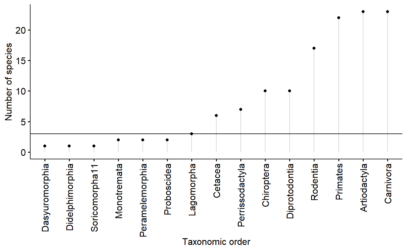
I will code each specis as being a member of an order w/ greater than 2 (“use”) or less than 2 species (“drop”)
orders$order.N.3.plus <- ifelse(orders$order.N >2,
                                "use",
                                "drop")
I’ll then merge this summary dataframe orders into the big dataframe
milk2 <- merge(milk,orders)
dim(milk)
#> [1] 130  23
dim(milk2)
#> [1] 130  25
Then I’ll select just the rows which can be used.
i.use <- which(milk2$order.N.3.plus == "use")

milk.working <- milk2[i.use, ]milk.working[which(milk.working$fat.log10 <0.5), ]
#> ord fam spp mass.fem
#> 60 Chiroptera Pteropodidae Pteropus poliocephalus 800
#> 73 Diprotodontia Potoroidae7 Potorous tridactylus 1047
#> 74 Diprotodontia Pseudocheiridae8 Pseudocheirus peregrinus 910
#> 82 Perrissodactyla Equidae Equus asinus 250000
#> 83 Perrissodactyla Equidae Equus burchellii 276000
#> 84 Perrissodactyla Equidae Equus ferus przewalskii 250000
#> 85 Perrissodactyla Equidae Equus zebra 262000
#> 86 Perrissodactyla Rhinocerotidae Diceros bicornis 884000
#> 87 Perrissodactyla Tapiridae Tapirus bairdii 300000
#> 89 Primates Atelidae12 Aloutta seniculus 5390
#> 90 Primates Atelidae12 Aloutta palliata 6400
#> 94 Primates Cercopithecidae Chlorocebus pygerythrus 5750
#> 98 Primates Cercopithecidae Miopithecus talapoin 1120
#> 104 Primates Hominidae Gorilla beringei beringei 90000
#> 105 Primates Lemuridae Eulemur fulvus 2500
#> 106 Primates Lemuridae Eulemur macaco 2250
#> 107 Primates Lemuridae Eulemur rubriventer 2000
#> 108 Primates Lemuridae Eulemur mongoz 1350
#> gest.mo lac.mo mass.litter repro.output dev.birth diet arid
#> 60 6.00 5.5 69.0 0.0900 2 herbivore no
#> 73 1.27 1.4 0.3 0.0003 0 omnivore yes
#> 74 3.50 7.3 0.6 0.0007 0 herbivore no
#> 82 11.97 13.0 29167.0 0.1200 3 herbivore yes
#> 83 12.16 10.8 32292.0 0.1200 3 herbivore yes
#> 84 11.50 10.5 30000.0 0.1200 3 herbivore yes
#> 85 12.02 10.0 30000.0 0.0100 3 herbivore yes
#> 86 16.12 19.9 34167.0 0.0400 2 herbivore yes
#> 87 13.17 12.0 9400.0 0.0300 3 herbivore no
#> 89 6.37 12.3 354.0 0.0700 2 herbivore no
#> 90 6.22 14.2 369.0 0.0600 2 herbivore no
#> 94 5.50 8.5 318.0 0.0600 2 omnivore no
#> 98 5.40 5.4 188.0 0.1700 2 omnivore no
#> 104 8.50 42.0 1600.0 0.0200 2 herbivore no
#> 105 4.02 5.0 85.0 0.0300 2 omnivore no
#> 106 4.37 5.2 79.0 0.0400 2 omnivore no
#> 107 4.28 3.3 86.0 0.0400 2 omnivore no
#> 108 4.29 5.1 71.0 0.0500 2 omnivore no
#> biome N fat gest.month lacat.mo prot sugar energy
#> 60 terrestrial 31 2.0 6.00 5.5 2.5 6.2 0.57
#> 73 terrestrial 5-Mar 3.0 1.27 1.4 10.0 14.0 1.41
#> 74 terrestrial >8 3.0 3.50 7.3 4.5 12.5 1.03
#> 82 terrestrial 9 1.8 11.97 13.0 1.7 5.9 0.50
#> 83 terrestrial 5 2.2 12.16 10.8 1.6 7.0 0.57
#> 84 terrestrial 14 1.5 11.50 10.5 1.6 6.7 0.50
#> 85 terrestrial 7 1.0 12.02 10.0 1.6 6.9 0.46
#> 86 terrestrial 11 0.2 16.12 19.9 1.4 6.6 0.36
#> 87 terrestrial 4 1.9 13.17 12.0 4.6 5.3 0.65
#> 89 terrestrial 7 1.1 6.37 12.3 1.9 6.6 0.47
#> 90 terrestrial 7 1.6 6.22 14.2 2.2 6.7 0.54
#> 94 terrestrial 4 3.1 5.50 8.5 1.6 8.5 0.71
#> 98 terrestrial 4 3.0 5.40 5.4 2.1 7.2 0.68
#> 104 terrestrial 7 1.9 8.50 42.0 1.4 6.8 0.52
#> 105 terrestrial 6 0.9 4.02 5.0 1.3 8.5 0.49
#> 106 terrestrial 7 1.1 4.37 5.2 1.5 8.4 0.52
#> 107 terrestrial 3 0.8 4.28 3.3 1.1 8.9 0.49
#> 108 terrestrial 4 0.7 4.29 5.1 1.3 7.9 0.45
#> genus fat.log10 mass.fem.log10 biome.diet order.N
#> 60 Pteropus 0.30103000 2.903090 terrestrial-herbivore 10
#> 73 Potorous 0.47712125 3.019947 terrestrial-omnivore 10
#> 74 Pseudocheirus 0.47712125 2.959041 terrestrial-herbivore 10
#> 82 Equus 0.25527251 5.397940 terrestrial-herbivore 7
#> 83 Equus 0.34242268 5.440909 terrestrial-herbivore 7
#> 84 Equus 0.17609126 5.397940 terrestrial-herbivore 7
#> 85 Equus 0.00000000 5.418301 terrestrial-herbivore 7
#> 86 Diceros -0.69897000 5.946452 terrestrial-herbivore 7
#> 87 Tapirus 0.27875360 5.477121 terrestrial-herbivore 7
#> 89 Aloutta 0.04139269 3.731589 terrestrial-herbivore 22
#> 90 Aloutta 0.20411998 3.806180 terrestrial-herbivore 22
#> 94 Chlorocebus 0.49136169 3.759668 terrestrial-omnivore 22
#> 98 Miopithecus 0.47712125 3.049218 terrestrial-omnivore 22
#> 104 Gorilla 0.27875360 4.954243 terrestrial-herbivore 22
#> 105 Eulemur -0.04575749 3.397940 terrestrial-omnivore 22
#> 106 Eulemur 0.04139269 3.352183 terrestrial-omnivore 22
#> 107 Eulemur -0.09691001 3.301030 terrestrial-omnivore 22
#> 108 Eulemur -0.15490196 3.130334 terrestrial-omnivore 22
#> order.N.3.plus
#> 60 use
#> 73 use
#> 74 use
#> 82 use
#> 83 use
#> 84 use
#> 85 use
#> 86 use
#> 87 use
#> 89 use
#> 90 use
#> 94 use
#> 98 use
#> 104 use
#> 105 use
#> 106 use
#> 107 use
#> 108 use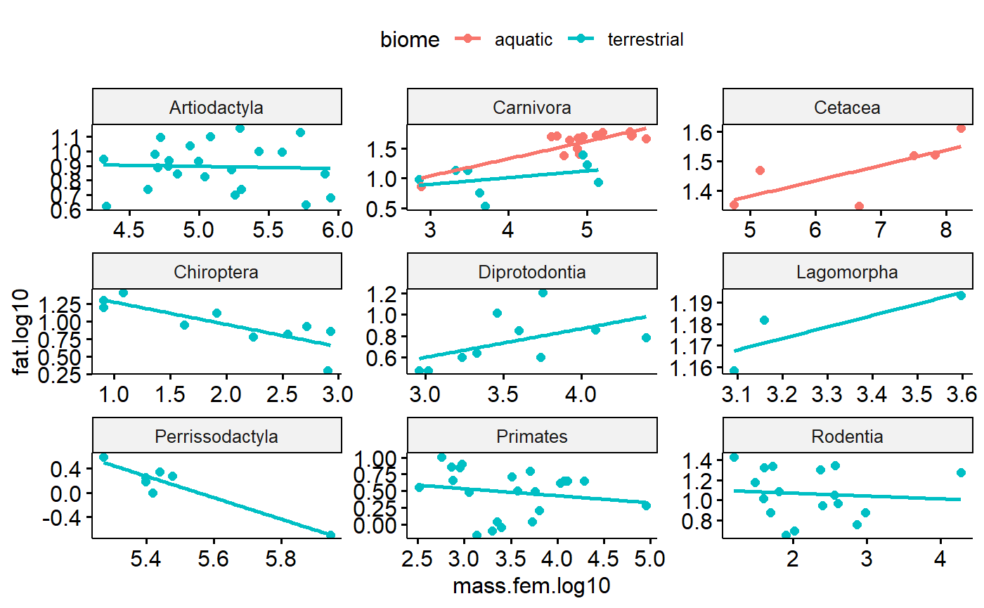
Build model
Diffrent slopes for each order
m.slopes <- lmer(fat.log10 ~ 1 +
                 (mass.fem.log10|ord) +
                 (1|fam) +
                 (1|genus),
data = milk.working)Compare models
ICtab(m.null,
      m.diet,
       m.mass,
       m.slopes,
       m.slopes.diet,
       m.slopes.x.diet,
      m.slopes.x.biome,
       type ="AICc",
       base = T,
       logLik = T,
       weights = T)
#>                  logLik AICc dLogLik dAICc df weight
#> m.slopes         -1.2   17.3  5.3     0.0  7  0.5409
#> m.null           -4.1   18.7  2.3     1.4  5  0.2649
#> m.diet           -2.9   20.7  3.5     3.4  7  0.0975
#> m.slopes.diet    -0.9   21.4  5.5     4.1  9  0.0699
#> m.slopes.x.biome -1.0   24.1  5.4     6.8  10 0.0182
#> m.mass           -6.4   25.6  0.0     8.3  6  0.0087
#> m.slopes.x.diet  -5.3   37.5  1.1    20.2  12 <0.001