e) The runFAC_multi() command: Running multiple FACs to explore the effects varying parameters
Nathan L. Brouwer
2022-03-07
e-the_runFAC_multi_command.RmdIntroduction
A major motivation for studying full-annual cycle population dynamics is to determine when during the annual cycle population limitation occurs. For example, a perennial question is whether habitat loss on the breeding grounds or wintering grounds is more important for population dynamics (TODO: CITE).
For standard density-independent (di) population models , such as matrix models (TODO: CITE) or integral projection models (TODO: CITE), there are analytical solutions that allow you to compare the importance of vital rates for population growth. These methods include sensitivity and elasticity analyses (TODO: CITE), as well as Life Table Response Experiments (LTRE; (TODO: CITE)). To carry out these analyses all that is required is the parameterized model and a program (such as R) that can do mathematical functions such as determinie what are known as the the eigenvalues of matrices. For an introduction to matrix models and eigenanlysis in R see … (TODO: CITE). For a general introduction to matrix models with worked examples see Morris and Doak 200x and the R package based on it popbio (TODO: CITE).
Density-dependent (dd) models are analyzed very differently than density-independent models (TODO: CITE). The add complexities of building and anlysing dd has made them relatively rare. Moreover, most dd models use functions similar to the classic logistic growth curve ((TODO: add figure of curve) to model have vital rates change as a function of density. For birds the primary form of density dependence is suspected to be due to the constrains imposed by a limited number of territories. This has been called site-dependence in the bird literature (TODo: cite Rodenhouse etc) and corresponds with what is called celing model of density depencence elsewhere (cite Morris and Doak, etc).
Complex dd models such as the one developed by Runge and Marra (2004) can not be assayed directly using analytical methods. Models such as this must be run repeatedly with different parameter values and the output of the model compared as conditions change. This requires running many indepdent models to equilibrium, each with slightly diffrent paramter values, storing the relevant output, and comparing the output. Runge and Marra (2004) graphically explored how
- varying breeding season and winter carrying capacity impacted breeding ground population size (Figures 28.3in the original paper),
- how breeding ground carrying capacity impacted breeding and winter population structure (28.4), and male dominance impacted the sex ratio (Figure 28.5), and
- the strength of carry-over effects impacted population size (Figure 28.6).
The redstart package implements and extends the analyses carried out by Runge and Marra (2004) using the function runFAC_multi(). This function allows you to run multiple FAC models each with different parameter values. The following vignette demonstrates the basic functionality of runFAC_multi(). Each of the analyses in Runge and Marra (2004) are then coverged in a seperate vignette.
Preliminaries
library(redstart)The runFAC_multi() function
runFAC_multi(param.grid = param_grid(), Ninit = c(10, 0, 10, 0), remakeFigure = NA, use.IBM = F, verbose = F, eq.tol = 6, …)
Recreate figures in the original paper
Figure 28.3: 3D surface
F28_3 <- runFAC_multi(eq.tol = 2,
                      verbose = F)
#> The dimension of the fully expanded dataframe is:
#> 100 by 30
#>
#> Model at equilibrium after 21 iterations
#>
#> Model at equilibrium after 21 iterations
#>
#> Model at equilibrium after 21 iterations
#>
#> Model at equilibrium after 21 iterations
#>
#> Model at equilibrium after 21 iterations
#>
#> Model at equilibrium after 21 iterations
#>
#> Model at equilibrium after 21 iterations
#>
#> Model at equilibrium after 21 iterations
#>
#> Model at equilibrium after 21 iterations
#>
#> Model at equilibrium after 24 iterations
#>
#> Model at equilibrium after 44 iterations
#>
#> Model at equilibrium after 44 iterations
#>
#> Model at equilibrium after 44 iterations
#>
#> Model at equilibrium after 44 iterations
#>
#> Model at equilibrium after 44 iterations
#>
#> Model at equilibrium after 44 iterations
#>
#> Model at equilibrium after 44 iterations
#>
#> Model at equilibrium after 44 iterations
#>
#> Model at equilibrium after 44 iterations
#>
#> Model at equilibrium after 24 iterations
#>
#> Model at equilibrium after 54 iterations
#>
#> Model at equilibrium after 54 iterations
#>
#> Model at equilibrium after 54 iterations
#>
#> Model at equilibrium after 54 iterations
#>
#> Model at equilibrium after 54 iterations
#>
#> Model at equilibrium after 54 iterations
#>
#> Model at equilibrium after 54 iterations
#>
#> Model at equilibrium after 54 iterations
#>
#> Model at equilibrium after 54 iterations
#>
#> Model at equilibrium after 24 iterations
#>
#> Model at equilibrium after 56 iterations
#>
#> Model at equilibrium after 61 iterations
#>
#> Model at equilibrium after 61 iterations
#>
#> Model at equilibrium after 61 iterations
#>
#> Model at equilibrium after 61 iterations
#>
#> Model at equilibrium after 61 iterations
#>
#> Model at equilibrium after 61 iterations
#>
#> Model at equilibrium after 61 iterations
#>
#> Model at equilibrium after 61 iterations
#>
#> Model at equilibrium after 24 iterations
#>
#> Model at equilibrium after 58 iterations
#>
#> Model at equilibrium after 64 iterations
#>
#> Model at equilibrium after 65 iterations
#>
#> Model at equilibrium after 65 iterations
#>
#> Model at equilibrium after 65 iterations
#>
#> Model at equilibrium after 65 iterations
#>
#> Model at equilibrium after 65 iterations
#>
#> Model at equilibrium after 65 iterations
#>
#> Model at equilibrium after 65 iterations
#>
#> Model at equilibrium after 24 iterations
#>
#> Model at equilibrium after 58 iterations
#>
#> Model at equilibrium after 66 iterations
#>
#> Model at equilibrium after 69 iterations
#>
#> Model at equilibrium after 69 iterations
#>
#> Model at equilibrium after 69 iterations
#>
#> Model at equilibrium after 69 iterations
#>
#> Model at equilibrium after 69 iterations
#>
#> Model at equilibrium after 69 iterations
#>
#> Model at equilibrium after 69 iterations
#>
#> Model at equilibrium after 24 iterations
#>
#> Model at equilibrium after 58 iterations
#>
#> Model at equilibrium after 67 iterations
#>
#> Model at equilibrium after 71 iterations
#>
#> Model at equilibrium after 72 iterations
#>
#> Model at equilibrium after 72 iterations
#>
#> Model at equilibrium after 72 iterations
#>
#> Model at equilibrium after 72 iterations
#>
#> Model at equilibrium after 72 iterations
#>
#> Model at equilibrium after 72 iterations
#>
#> Model at equilibrium after 24 iterations
#>
#> Model at equilibrium after 58 iterations
#>
#> Model at equilibrium after 69 iterations
#>
#> Model at equilibrium after 72 iterations
#>
#> Model at equilibrium after 74 iterations
#>
#> Model at equilibrium after 74 iterations
#>
#> Model at equilibrium after 74 iterations
#>
#> Model at equilibrium after 74 iterations
#>
#> Model at equilibrium after 74 iterations
#>
#> Model at equilibrium after 74 iterations
#>
#> Model at equilibrium after 24 iterations
#>
#> Model at equilibrium after 58 iterations
#>
#> Model at equilibrium after 69 iterations
#>
#> Model at equilibrium after 73 iterations
#>
#> Model at equilibrium after 75 iterations
#>
#> Model at equilibrium after 76 iterations
#>
#> Model at equilibrium after 76 iterations
#>
#> Model at equilibrium after 76 iterations
#>
#> Model at equilibrium after 76 iterations
#>
#> Model at equilibrium after 76 iterations
#>
#> Model at equilibrium after 24 iterations
#>
#> Model at equilibrium after 58 iterations
#>
#> Model at equilibrium after 69 iterations
#>
#> Model at equilibrium after 74 iterations
#>
#> Model at equilibrium after 76 iterations
#>
#> Model at equilibrium after 78 iterations
#>
#> Model at equilibrium after 78 iterations
#>
#> Model at equilibrium after 78 iterations
#>
#> Model at equilibrium after 78 iterations
#>
#> Model at equilibrium after 78 iterations
runFAC_multi produces a list with two elements.
is(F28_3)
#> [1] "list"   "vector"
length(F28_3)
#> [1] 2
One holds the output for the original model of Runge and Marra (rmFAC; multiFAC.out.df.RM), while the other holds the output for from a model with individual-based submodels (ibFAC; multiFAC.out.df.IB:’data.frame). We’ll focus on rmFAC.
str(F28_3, 1)
#> List of 2
#>  $ multiFAC.out.df.RM:'data.frame':  100 obs. of  53 variables:
#>  $ multiFAC.out.df.IB:'data.frame':  100 obs. of  41 variables:
The rmFAC element is a dataframe.
is(F28_3$multiFAC.out.df.RM)
#> [1] "data.frame" "list"       "oldClass"   "vector"
This dataframe contains information on the output of dozens of individual runs of the FAC model to equilibrium, so it very large
dim(F28_3$multiFAC.out.df.RM)
#> [1] 100  53
There are 23 rows for various output such as the population sizes and sex ratios. There are 100 rows.
str(F28_3$multiFAC.out.df.RM,1)
#> 'data.frame':    100 obs. of  53 variables:
#>  $ B.mc          : num  0.371 2.702 2.702 2.702 2.702 ...
#>  $ B.mk          : num  0 0 0 0 0 0 0 0 0 0 ...
#>  $ B.md          : num  0 0 0 0 0 0 0 0 0 0 ...
#>  $ B.fc          : num  0.341 2.597 2.597 2.597 2.597 ...
#>  $ B.fk          : num  0 0 0 0 0 0 0 0 0 0 ...
#>  $ W.mg          : num  0.407 0.838 0.838 0.838 0.838 ...
#>  $ W.mp          : num  0.121 3.086 3.086 3.086 3.086 ...
#>  $ W.fg          : num  0.157 0.162 0.162 0.162 0.162 ...
#>  $ W.fp          : num  0.348 3.682 3.682 3.682 3.682 ...
#>  $ P.cgg         : num  0.337 0.045 0.045 0.045 0.045 ...
#>  $ P.cgp         : num  0.52 0.187 0.187 0.187 0.187 ...
#>  $ P.cpg         : num  0 0 0 0 0 0 0 0 0 0 ...
#>  $ P.cpp         : num  0.142 0.768 0.768 0.768 0.768 ...
#>  $ P.kgg         : num  0 0 0 0 0 0 0 0 0 0 ...
#>  $ P.kgp         : num  0 0 0 0 0 0 0 0 0 0 ...
#>  $ P.kpg         : num  0 0 0 0 0 0 0 0 0 0 ...
#>  $ P.kpp         : num  0 0 0 0 0 0 0 0 0 0 ...
#>  $ y.mc          : num  0.246 1.87 1.87 1.87 1.87 ...
#>  $ y.mk          : num  0 0 0 0 0 0 0 0 0 0 ...
#>  $ y.fc          : num  0.246 1.87 1.87 1.87 1.87 ...
#>  $ y.fk          : num  0 0 0 0 0 0 0 0 0 0 ...
#>  $ A.G.mc        : logi  NA NA NA NA NA NA ...
#>  $ A.G.mk        : logi  NA NA NA NA NA NA ...
#>  $ A.G.md        : logi  NA NA NA NA NA NA ...
#>  $ A.G.y.mc      : logi  NA NA NA NA NA NA ...
#>  $ A.G.y.mk      : logi  NA NA NA NA NA NA ...
#>  $ A.G.fc        : logi  NA NA NA NA NA NA ...
#>  $ A.G.fk        : logi  NA NA NA NA NA NA ...
#>  $ A.G.y.fc      : logi  NA NA NA NA NA NA ...
#>  $ A.G.y.fk      : logi  NA NA NA NA NA NA ...
#>  $ A.P.mc        : logi  NA NA NA NA NA NA ...
#>  $ A.P.mk        : logi  NA NA NA NA NA NA ...
#>  $ A.P.md        : logi  NA NA NA NA NA NA ...
#>  $ A.P.y.mc      : logi  NA NA NA NA NA NA ...
#>  $ A.P.y.mk      : logi  NA NA NA NA NA NA ...
#>  $ A.P.fc        : logi  NA NA NA NA NA NA ...
#>  $ A.P.fk        : logi  NA NA NA NA NA NA ...
#>  $ A.P.y.fc      : logi  NA NA NA NA NA NA ...
#>  $ A.P.y.fk      : logi  NA NA NA NA NA NA ...
#>  $ error1        : logi  NA NA NA NA NA NA ...
#>  $ error2        : logi  NA NA NA NA NA NA ...
#>  $ gamma.i       : num  5 5 5 5 5 5 5 5 5 5 ...
#>  $ c.i           : num  1 1 1 1 1 1 1 1 1 1 ...
#>  $ K.bc.i        : num  1 112 223 334 445 556 667 778 889 1000 ...
#>  $ K.wg.i        : num  1 1 1 1 1 1 1 1 1 1 ...
#>  $ B.m.tot       : num  0.371 2.702 2.702 2.702 2.702 ...
#>  $ B.m.tot.no.d  : num  0.371 2.702 2.702 2.702 2.702 ...
#>  $ B.f.tot       : num  0.341 2.597 2.597 2.597 2.597 ...
#>  $ sex.ratio     : num  1.09 1.04 1.04 1.04 1.04 ...
#>  $ sex.ratio.no.d: num  1.09 1.04 1.04 1.04 1.04 ...
#>  $ B.tot         : num  0.712 5.3 5.3 5.3 5.3 ...
#>  $ B.tot.no.d    : num  0.712 5.3 5.3 5.3 5.3 ...
#>  $ variable      : int  1 2 3 4 5 6 7 8 9 10 ...
Each rows is a single run of the model. runFAC_multi() is designed to run the model over multiple combinations of parametrs. A principle output is a 3D surface plot where the x and y axes are two parameters varied between runs of the model and the z (vertical axis) is a state of interest when the model is at equilibrium, such as the equilibirum summer population size.
Plot the 3D surface.
par(mfrow = c(1,1))
plot_Fig28_3(F28_3$multiFAC.out.df.RM)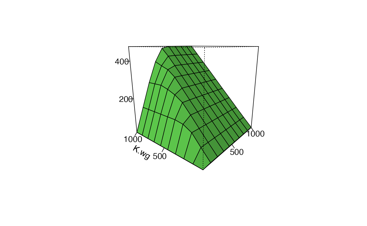
Figure 28.4
Create the intial range of the parameters
The param_ranges() function can be used to create ranges (minimum and maxiumum) of parameters that can then be subsequently explored using runFAC_multi(). This is the first step, followed by generating sequences of numbers between the min and the max. param_ranges() is set up to take as arguements different scenarios (scenario = … ) or figures (figure = …) defined by Runge and Marra and to produce the combinations of parameters used in that paper. In general one or two parameters are varied and all the others are kept constant.
We can set up the parameters for Figures 28.3 and 28.4 like this
F28.3.range <- param_ranges(figure = 28.3)
F28.4.range <- param_ranges(figure = 28.4)
In this figure K.bc was varied from 100 to 600 and all other parameters kept constant.
head(F28.4.range)
#>          min   max
#> gamma  5e+00 5e+00
#> co.    1e+00 1e+00
#> K.bc   1e+00 6e+02
#> K.bk   1e+04 1e+04
#> K.wg   9e+02 9e+02
#> S.w.mg 8e-01 8e-01
Turn any varying parameters into sequence
Once the minimum and maxium are set the actual sequence of numbers can be made. This
For Figure 28.4 breding ground carrying capacity is varied from 100 to 600, so we want a vector of numbers, say 100, 200, 300, 400, 500, 600.
For Figure 28.3 breding ground carrying capacity is varied from 1 to 1000, and also winter carrying capacity is varied from 1 to 100.
We make a list the has all the parameters we need
F28.3.seq <- param_seqs(F28.3.range)
F28.4.seq <- param_seqs(F28.4.range)
This is a list
is(F28.4.seq)
#> [1] "list"   "vector"
There is one element for each input parameter
length(F28.4.seq)
#> [1] 30
If a parameter does not need to be varied a single value appears in its slot. Otherwise a vector. For figure 28.4 there is just one parameter that varies
head(F28.4.seq)
#> $gamma
#> [1] 5
#>
#> $co.
#> [1] 1
#>
#> $K.bc
#>  [1]   1.00000  67.55556 134.11111 200.66667 267.22222 333.77778 400.33333
#>  [8] 466.88889 533.44444 600.00000
#>
#> $K.bk
#> [1] 10000
#>
#> $K.wg
#> [1] 900
#>
#> $S.w.mg
#> [1] 0.8
For figure 28.3 there are two
head(F28.3.seq)
#> $gamma
#> [1] 5
#>
#> $co.
#> [1] 1
#>
#> $K.bc
#>  [1]    1  112  223  334  445  556  667  778  889 1000
#>
#> $K.bk
#> [1] 10000
#>
#> $K.wg
#>  [1]    1  112  223  334  445  556  667  778  889 1000
#>
#> $S.w.mg
#> [1] 0.8
Expand parameters into a grid
Once the parameters have been defined a set of all possible parameter combinations needs to be created. This is essentially a grid of all possible value. (The shape isn’t a square grid, but takes its name from the use of R’s expand.grid function)
For figure 28.4 only one parameter is varied.
F28.4.grid <- param_grid(param.seqs = F28.4.seq)
#> The dimension of the fully expanded dataframe is:
#> 10 by 30
Figure 28.3 is much larger because two parameters are varied.
F28.3.grid <- param_grid(param.seqs = F28.3.seq)
#> The dimension of the fully expanded dataframe is:
#> 100 by 30
The output is a dataframe
is(F28.4.grid)
#> [1] "data.frame" "list"       "oldClass"   "vector"
Each row of the dataframe contains all the parameters needed for a single run of the model.
head(F28.4.grid)[,1:10]
#>   gamma co.      K.bc  K.bk K.wg S.w.mg S.w.mp S.w.fg S.w.fp S.m.mg
#> 1     5   1   1.00000 10000  900    0.8    0.8    0.8    0.8    0.9
#> 2     5   1  67.55556 10000  900    0.8    0.8    0.8    0.8    0.9
#> 3     5   1 134.11111 10000  900    0.8    0.8    0.8    0.8    0.9
#> 4     5   1 200.66667 10000  900    0.8    0.8    0.8    0.8    0.9
#> 5     5   1 267.22222 10000  900    0.8    0.8    0.8    0.8    0.9
#> 6     5   1 333.77778 10000  900    0.8    0.8    0.8    0.8    0.9
Each row of data will be fed in the runFAC() function and the model run until an equilibirum is reached.
Run multiple FACs accross the parameters
We can run the grid to equilibrium with runFAC_multi().
F28.4.FAC <- runFAC_multi(param.grid = F28.4.grid,
                             verbose = F,
                             eq.tol =6,
                             Ninit = c(100, 0, 100, 0))
#>
#> Model at equilibrium after 57 iterations
#>
#> Model at equilibrium after 40 iterations
#>
#> Model at equilibrium after 51 iterations
#>
#> Model at equilibrium after 57 iterations
#>
#> Model at equilibrium after 42 iterations
#>
#> Model at equilibrium after 53 iterations
#>
#> Model at equilibrium after 58 iterations
#>
#> Model at equilibrium after 137 iterations
#>
#> Model at equilibrium after 122 iterations
#>
#> Model at equilibrium after 122 iterations
Plot Figure 28.4
Different kinds of figures require different set up and so there are specific functions for each figure. Figure 28.3 is made with function plot_Fig28_3(). Figure 28.4 has its own function.
plot_Fig28_4(F28.4.FAC$multiFAC.out.df.RM)