7.2 Data pre-loaded in R
R comes with a number of datasets ready to use. A famous dataset frequently used in statistics is a set of measurements made on three species of irises and used to demonstrate some statistical principles by geneticist and statistician R.A. Fisher.
We can put the iris dataset into R’s working memory using the data() command
data(iris)We can see these data simply by type the word “iris” in the console and pressing enter. The dataset is too big for the screen probably and you’ll just see a bunch of numbers flash by. You can get just a glimpse of the data by using the head() command, which will show you the first six or so rows of data.
head(iris)## Sepal.Length Sepal.Width Petal.Length Petal.Width Species
## 1 5.1 3.5 1.4 0.2 setosa
## 2 4.9 3.0 1.4 0.2 setosa
## 3 4.7 3.2 1.3 0.2 setosa
## 4 4.6 3.1 1.5 0.2 setosa
## 5 5.0 3.6 1.4 0.2 setosa
## 6 5.4 3.9 1.7 0.4 setosa(You can all use the tail() command to see the last 6 rows if you want.)
We can see that there are five rows of data. Three contain information about the length and width of the parts of the flower (Sepals and Petals) and the last holds the names of the species.
We can get a sense for these numbers by using the summary() command on the data, which will give us the mean and other summary statistics
summary(iris)## Sepal.Length Sepal.Width Petal.Length Petal.Width
## Min. :4.300 Min. :2.000 Min. :1.000 Min. :0.100
## 1st Qu.:5.100 1st Qu.:2.800 1st Qu.:1.600 1st Qu.:0.300
## Median :5.800 Median :3.000 Median :4.350 Median :1.300
## Mean :5.843 Mean :3.057 Mean :3.758 Mean :1.199
## 3rd Qu.:6.400 3rd Qu.:3.300 3rd Qu.:5.100 3rd Qu.:1.800
## Max. :7.900 Max. :4.400 Max. :6.900 Max. :2.500
## Species
## setosa :50
## versicolor:50
## virginica :50
##
##
## Note that the last column doesn’t contain numbers but rather names, so R counts up how many of each species name there is.
If we want to be reminded of the names of each column we can use the names() function
names(iris)## [1] "Sepal.Length" "Sepal.Width" "Petal.Length" "Petal.Width"
## [5] "Species"Looking at R data in the console isn’t always very easy, so one thing you can do is use the View() command. This will bring up the data in a spreadsheet like viewer as a new tab in the script editor, similar to this.
pander::pander(iris[1:10,])| Sepal.Length | Sepal.Width | Petal.Length | Petal.Width | Species |
|---|---|---|---|---|
| 5.1 | 3.5 | 1.4 | 0.2 | setosa |
| 4.9 | 3 | 1.4 | 0.2 | setosa |
| 4.7 | 3.2 | 1.3 | 0.2 | setosa |
| 4.6 | 3.1 | 1.5 | 0.2 | setosa |
| 5 | 3.6 | 1.4 | 0.2 | setosa |
| 5.4 | 3.9 | 1.7 | 0.4 | setosa |
| 4.6 | 3.4 | 1.4 | 0.3 | setosa |
| 5 | 3.4 | 1.5 | 0.2 | setosa |
| 4.4 | 2.9 | 1.4 | 0.2 | setosa |
| 4.9 | 3.1 | 1.5 | 0.1 | setosa |
Note, however, that unlike a spreadsheet you cannot edit the data.
If you want to know more about a package, you can look at its help file, eg “?iris.” These will often give you a fair bit of detail about what each column means, where the data are from, and may even have examples R functions applied to the data (though these can be rather obtuse, as is the case for the iris data).
7.2.1 Preview: Plotting boxplots
Plotting will be covered in depth in a subsequent exercise, but here’s a glimpse of how we plot things in R:
plot(Petal.Length ~ Species, data = iris)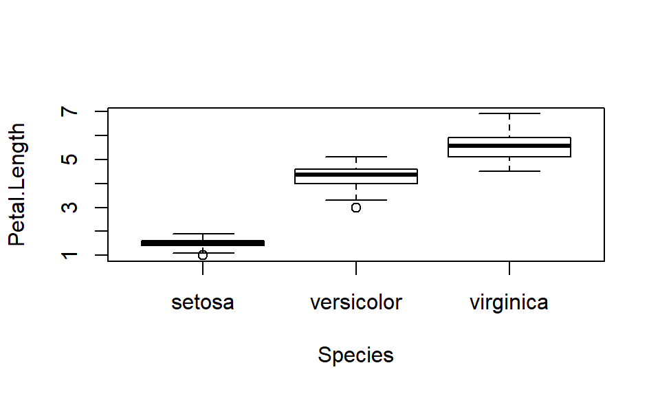
This code creates a series of boxplots of the petal lengths of each species of flower.