R for Ecological Data Science: A Gentle Introduction

7.6 Loading data from an R script

So far we have only looked at dataset that are already formatted into dataframe by somebody for us. Now we want to look at how to set up datasets ourselves. When datasets are small its possible to enter them more or less directly into R by typing out all of the numbers in a script. This only works well for when datasets are small; even when datasets are small its best to keep them separate from your R code in a spreadsheet file. However, its useful to know how to load data this way; even when an exercise in this book loads data from a package or spreadsheet I will also often include the code to load it directly just in case there is an issue with download the package or file.

7.6.1 The eagles have landed - in your R workspace

In a subsequent exercise we will practice using data on the number of eagles in Pennsylvania and other states in the USA. We can load this data into R by making R objects, and then turning these objects into a dataframe.

7.6.1.1 Step one: Build R objects

First, we’ll use the assignment operator (“<-”) to create an R object called “year” that lists the years from 1980 through 2015 for which the number breeding pairs of eagles in Pennsylvania, USA, is known.

year <- c(1980,1981,1982,1983,1984,1985,1986,1987,1988,1989,
          1990,1991,1992,1993,1994,1995,1996,1997,1998,1999,
          2000,2001,2002,2003,2004,2005,2006,2007,2008,2009,
          2010,2011,2012,2013,2014,2015,2016)

A quick trick to do this much fast is

year <- c(1980:2016)

Second, we’ll create an object called “eagles” with the number of breeding pairs (male and females paired up for making baby eagles) recorded each year. Note that most years in the 1980s are skipped because there is not data available. When data are missing we use NA. (Note that this is just NA, with not quotes around it).

eagles <-  c(3, NA, NA, NA, NA, NA, NA,NA,NA,NA,
             7,  9, 15, 17, 19, 20, 20,23,29,43,
             51,55, 64, 69, NA, 96,100,NA,NA,NA,
             NA,NA, NA, NA,252,277, NA)

7.6.1.2 Step two: Build dataframe

We can then turn these two separate R objects into a dataframe

eagle.df <-data.frame(year, eagles)

7.6.2 Looking at the eagle data

We can check that we have this R object by using the ls() command.

ls()

## [1] "crabs"    "eagle.df" "eagles"   "iris"     "msleep"   "my.abc"  
## [7] "my.mean"  "x"        "year"

And we can confirm that its a dataframe using is()

is(eagle.df)

## [1] "data.frame" "list"       "oldClass"   "vector"

summary() will give us basic info on PA’s eagles

summary(eagle.df)

##       year          eagles      
##  Min.   :1980   Min.   :  3.00  
##  1st Qu.:1989   1st Qu.: 18.00  
##  Median :1998   Median : 29.00  
##  Mean   :1998   Mean   : 61.53  
##  3rd Qu.:2007   3rd Qu.: 66.50  
##  Max.   :2016   Max.   :277.00  
##                 NA's   :18

Note that in the “eagles” columns it tells you the number of NAs (missing values). The summary() readout quickly tells us that the eagle population has changed dramatically.

7.6.2.1 Preview: Plotting the Eagle D

We can plot the data in ggplot2 using qplot(). However, there is an excellent package that adds additional functionality to ggplot called ggpubr. This is fairly common in R: you have packages that add functions to R, and packages that add functions to other packages.

We can install ggpubr using install.packages(). Note that the name of the package, ggpubr, is in quotes.

install.packages("ggpubr")

ggpubr requires another package, magrittr, which R tells you about in red text. When a package requires another package, its called a dependency because one package relies on another. ggpubr has magrittr as a dependency; ggpubr modifies ggplot2, so ggpubr has ggplot2 as a dependency.

Occasionally you might try to load a package and it won’t automatically install or download the dependency, usually because its not yet downloaded. If this happens with magrittr we would just have to download it using “install.packages(”magrittr“)”.

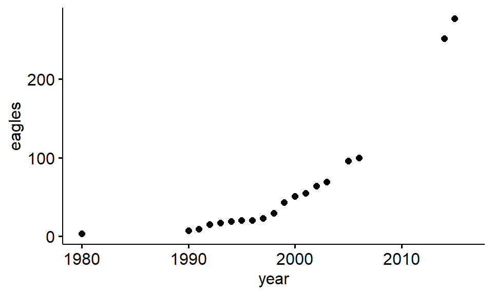
Once we have ggpubr loaded we can plot the eagle data using the handy function ggscatter()

ggscatter(dat = eagle.df, y = "eagles", x= "year")