7.5 Load data from an external R package

Many packages have to be explicitly downloaded and installed in order to use their functions and datasets. Note that this is a two step process: 1. Download package from internet 1. Explicitly tell R to load it

7.5.1 Step 1: Downloading packages

There are a number of ways to install packages. One of the easiest is to use install.packages(). Note that it might be better to call this “download.packages” since after you install it, you also have to load it!

Well download a package used for plotting called ggplot2, which stands for “Grammar of graphics”

install.packages("ggplot2")

Often when you download a package you’ll see a fair bit of red text. Usually there’s nothing of interest hear, but sometimes you need to read over it for hints about why something didn’t work.

7.5.2 Step 2: Explicitly loading a package

The install.packages() functions just saves the package software to R; now you need to tell R “I want to work with the package”. This is done using the library() function. (Its called library because another name for packages is libraries)

library(ggplot2)

ggplot2 has a dataset called “msleep” which has information on the relationship between the typical size of a species and its brain weight, among other things

We load the data actively into R’s memory using data(), and can look at the column names using names()

data(msleep)
names(msleep)

##  [1] "name"         "genus"        "vore"         "order"       
##  [5] "conservation" "sleep_total"  "sleep_rem"    "sleep_cycle" 
##  [9] "awake"        "brainwt"      "bodywt"

We can now explore this data set as before using summary(), str(), etc.

Another useful command when you are working with a new dataset is dim(). This tells you the dimension of the dataframe

dim(msleep)

## [1] 83 11

7.5.3 Preview: plotting with ggplot2

ggplot2 is a powerful plotting tool that has become standard among scientists, data scientists, and even journalists. Here’s a quick way to make a plot in ggplot2 using its qplot() function (qplot = quick plot, not to be confused with qqplot). Note that the qplot() function only works if you have ggplot2 downloaded and installed.

A powerful aspect of ggplot is the fact that it can easily be used to modify plots. Here, we use the arguement “color =” to color code the data points based on their IUCN red list status.

qplot(y = brainwt, x = bodywt, data = msleep, color = conservation)

## Warning: Removed 27 rows containing missing values (geom_point).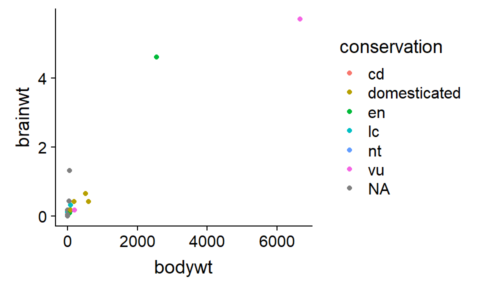

The animals in this data vary in size from mice to elephants and so a lot of the data points are scrunched together. A trick to make this easier to see is to take the log of the brainwt and bodywt variable. In R, we can do this on the fly like this using the log() command

qplot(y = log(brainwt), x = log(bodywt), data = msleep, color = conservation)

## Warning: Removed 27 rows containing missing values (geom_point).