15.2 Scatterplots: 2 Continuous Variables

In this lab we’ll explore how to make scatterplots using the qplot() function in ggplot2.

15.2.1 R Preliminaries

• We’ll use the qplot() function in the ggplot package
• The cowplot package provides nice deafults for ggplot IMHO

15.2.2 Scatterplot of Iris data

• Let’s make a scatter plot, where we plot two continous, numeric variables against each other
• that is, both x and y variables are numbers; not categories

I’ve forgotten the names of all the iris variables, so I’ll use the names() command to see what they are

names(iris)

I’ll plot the sepals against the petals

qplot(y = Sepal.Length,
      x = Petal.Length, 
      data = iris)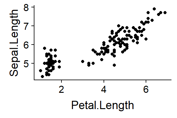

Figure 15.1: Sepals vs. Petals

15.2.3 Scatter plot of mammal brain data

Let’s look at another dataset

15.2.3.1 Preliminaries

Get the data from the ggplot2 package

data(msleep)

15.2.3.2 Look at the data

dim(msleep) #How much data is there?

head(msleep) #What does the data look like

summary(msleep) #Summary of the data

There are a number of “categorical” varibles in this dataset

• genus
• vore = carnivore, omnivore et
• order = taxonomic order
• conservation = conservation status (endangered, etc)

For some reason they don’t load as “factor” variables (better known as categorical or grouping variables, but called “Factors” in R-land)

We can make these factors using the factor() command

msleep$vore <- factor(msleep$vore)

Now see what happens when you call summary()

summary(msleep)

Do the same for “order”"

msleep$order <- factor(msleep$order)

summary(msleep)

And “conservation”

msleep$conservation <- factor(msleep$conservation)

summary(msleep)

15.2.4 Make a basic scatterplot

qplot(y = sleep_total,
      x = brainwt, 
      data = msleep)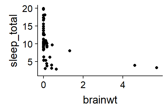

Figure 15.2: Mammal sleep, raw data

That looks really really ugly. It will work better if we “log transform the axes”

qplot(y = log(sleep_rem),
      x = log(brainwt), 
      data = msleep)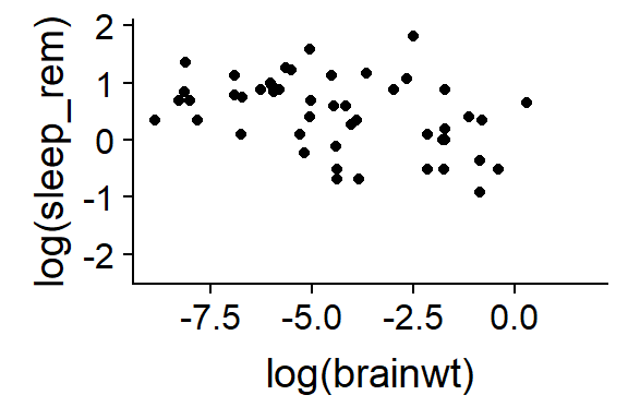

Figure 15.3: Mammal sleep, logged data

Things get logged all the time in stats. We’ll talk more about that later.

15.2.5 Add color coding to scatterplot

qplot(y = log(sleep_rem),
      x = log(brainwt), 
      data = msleep,
      color = vore)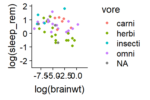

Figure 15.4: Add colors with color =

15.2.6 Add color & shape coding to scatterplot

qplot(y = log(sleep_rem),
      x = log(brainwt), 
      data = msleep,
      color = vore,
      shape = vore)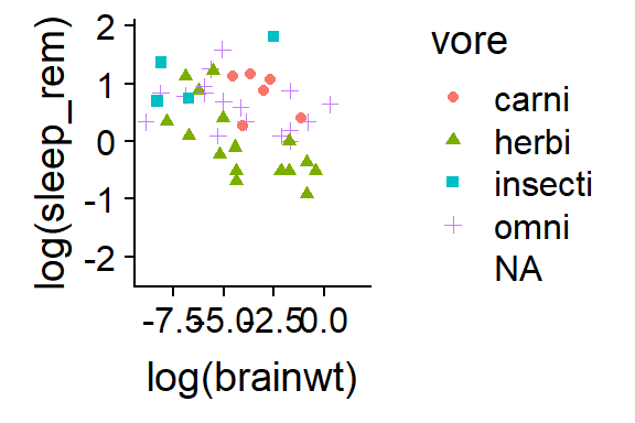

Figure 15.5: Add shapes with shape =

15.2.7 Put diffetrent “vores” in seperate panels

• Seperate panels can be made using the “facet” arguement withing qplot

qplot(y = log(sleep_rem),
      x = log(brainwt), 
      data = msleep,
      color = vore,
      shape = vore,
      facets = vore ~ .)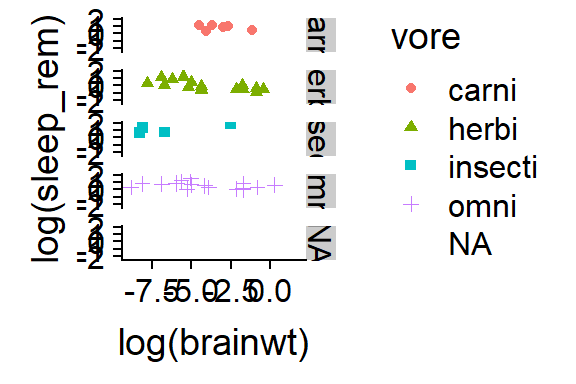

Figure 15.6: Split into different panels w/ facets =

15.2.8 Add a “trend line”" to a scatterplot

• Add the geom_smooth() function after the initial qplot() command
• This works best if we remove the “color = vore” command, but you can see what happens if you leave it

qplot(y = log(sleep_rem),
      x = log(brainwt), 
      data = msleep) +
  geom_smooth()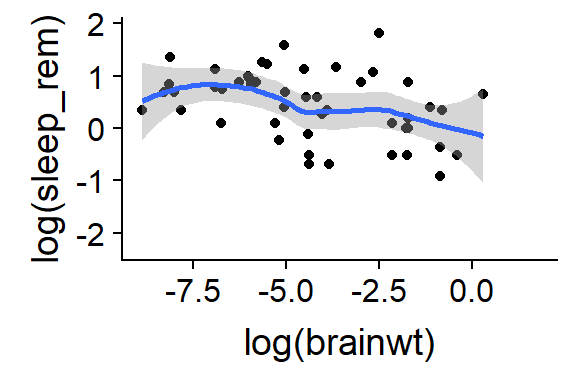

(#fig:last.chnk.sxn3.ch3)Add trendline with + geom_smooth()

15.2.9 Challenge: Modify mammal brain code

Modify the mamal bran code to do the following things

• Change the axes labels (eg “+ ylab(‘y axis’)”)
• Add a title (eg " + ggtitle(‘…’)“)
• Use names(msleep) to see what other varibles are in the dataset
• Use summary(msleep) to whether they are continous or categorical
• Pick another continous variable and plot it instead of sleep_total
• Try this with and without logging using the log() command

In this section we will tackle a typical data analysis problem: determining if two groups, such as organisms or drug treatments, an be considered statistically different from each other. We will use data from a paper titled “Sperm competition and the evolution of precopulatory weapons: Increasing male density promotes sperm competition and reduces selection on arm strength in a chorusing frog” by Buzatto et al (2015).

The end goal is to compare the size of the arms on female and male frogs. First, though, we will get to know the data by calculating summary statistics and making exploratory graphs. We will then carry out a t-test and grapple with with the meaning and interpretation of the output Finally, we’ll explore how best to plot the output of a t-test.

Section outline:

1. Data exploration with summary statistics
2. Graphical data exploration with boxplots
3. Plotting means and measures of variation and precision
4. T-tests
5. Plotting the output of a t-test